Module 3 · Training and Generation
Chapter 13 of 17 Run it in your browser

Chapter 13: The Training Loop¶

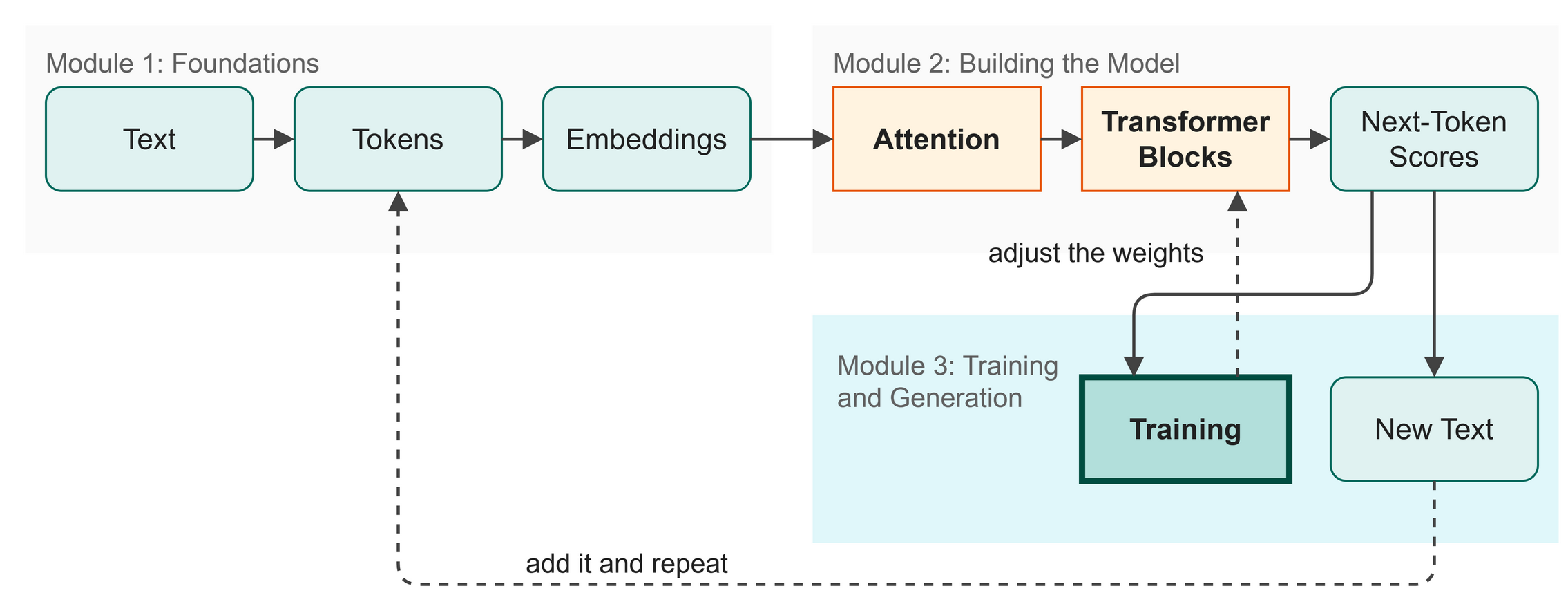Name: Teach Your Computer to Write: Build and Train an LLM from Zero
Author: Truong (Jack) Luu

You are here: Training Figure 13.1: The model makes predictions, measures its error, and adjusts its weights to improve.

Everything we have built so far comes down to this chapter. With our data batched and ready from Chapter 12, we have a model that can guess the next character, but right now, its guesses are no better than chance. In this chapter, we will write the loop that teaches it the patterns of the text it reads.

In this chapter you will:

Understand gradient descent as walking down a hill.
See what the learning rate does, by measuring three of them.
Build the four-step training loop.
Watch the model learn in real time, and read what its loss means.

Words to Know

Optimizer: The algorithm that updates the model's weights. We use Adam, a popular and steady choice.
Gradient: The direction we need to move our weights to increase the error. We move in the opposite direction to decrease it.
Backpropagation: The mathematical process of calculating the gradient for every single weight in the model.
Learning Rate: How far the optimizer moves the weights on each step. If it is too small, training crawls, and if it is too large, it can overshoot.

Theory¶

Walking Down the Hill¶

How does the model improve? Imagine you are blindfolded on a bumpy hillside, and you want to reach the very bottom (the lowest possible loss).

You can't see the whole hill, but you can feel the slope of the ground right under your feet. If the ground slopes up to your right, you know you should take a step to your left.

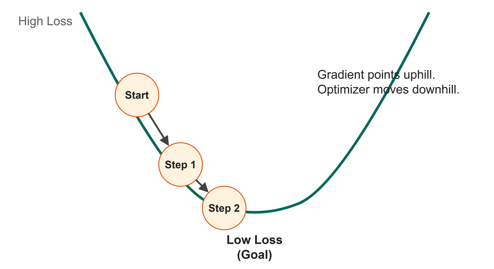Gradient descent as walking down a hill Figure 13.2: The optimizer takes small steps down the loss landscape to find the best weights.

This is gradient descent (Figure 13.2). The slope under your feet is the gradient, calculated by backpropagation, and taking a small step downhill is the optimizer updating the weights.

The Four-Step Loop¶

Training is a repetitive cycle that we run thousands of times (Figure 13.3):

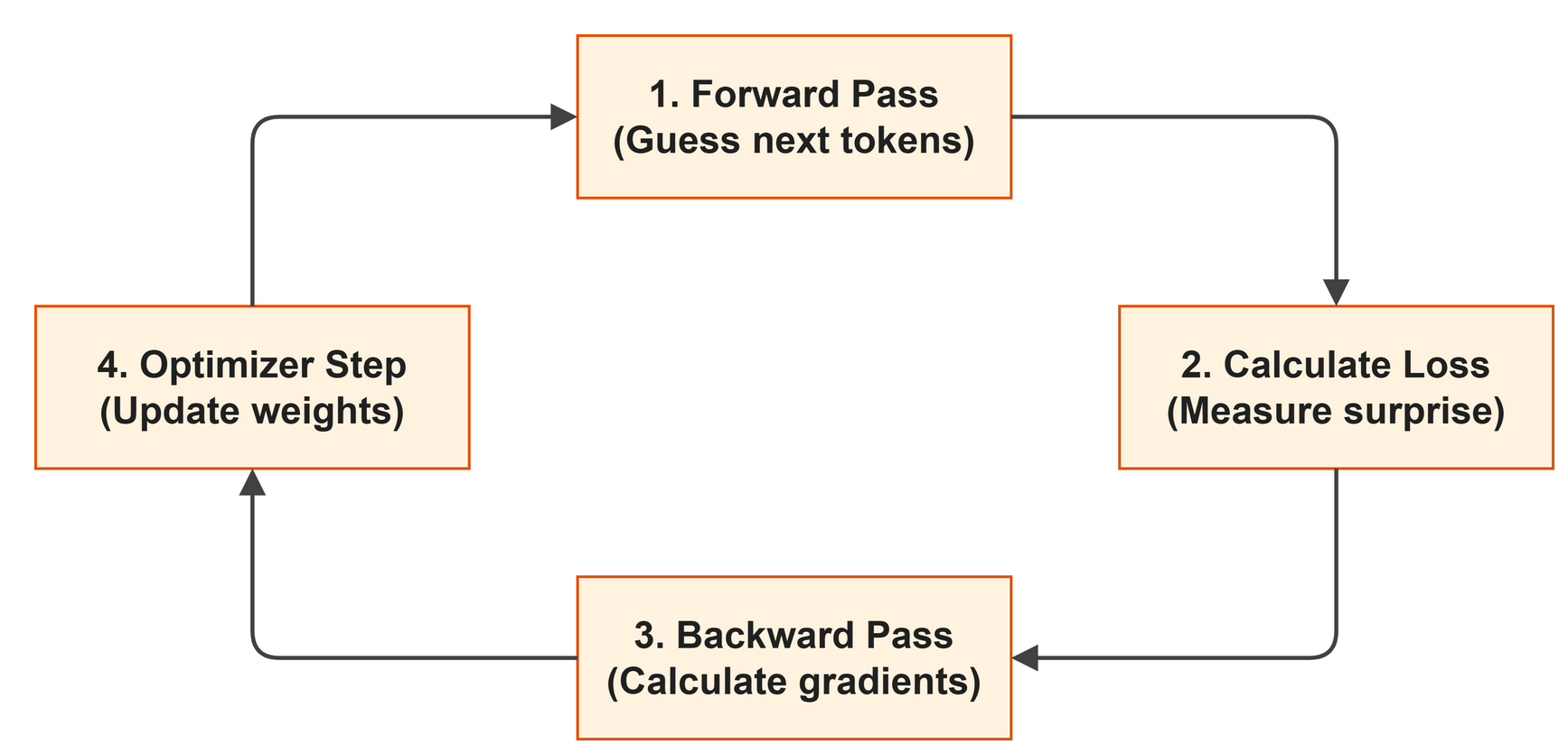The training loop cycle Figure 13.3: The four steps of the training loop.

Forward Pass: We pass a batch of data through the model to get its predictions.
Calculate Loss: We compare the predictions to the correct targets using cross-entropy.
Backward Pass: PyTorch automatically works out the gradient for every weight in the model (loss.backward()). The part of PyTorch that does this is called autograd.
Optimizer Step: The optimizer adjusts the weights slightly in the right direction (optimizer.step()).

How Big Should the Step Be?¶

Gradient descent tells you which way is downhill. It does not tell you how far to walk. That distance is the learning rate, and it is the one number beginners most often get wrong.

Our config sets it to 0.0003. Where does that come from? Rather than take it on faith, train the same model three times from the same starting weights, changing only the learning rate:

src/examples/ch13_learning_rate.py
for lr in (3e-3, 3e-4, 3e-5):
    torch.manual_seed(42)                       # same starting weights every time
    model = GPT(GPTConfig())
    optimizer = torch.optim.Adam(model.parameters(), lr=lr)

Terminal

$ python src/examples/ch13_learning_rate.py
lr=0.003    start 4.33  after 150 steps 2.35
lr=0.0003   start 4.33  after 150 steps 2.60
lr=3e-05    start 4.33  after 150 steps 3.31

The bottom row is the lesson most people need. At 0.00003 the steps are so small that after 150 steps the model has barely moved. Its loss is 3.31, when random guessing is 4.17. It is learning, just far too slowly to be useful. If your loss is falling but crawling, suspect the learning rate before you suspect anything else.

The top row is more interesting, because it does not say what you might expect. Ten times the learning rate learned faster here, reaching 2.35 while our chosen rate reached 2.60. So why does the book not use it?

Because 150 steps is not 3,000. A large step size is a gamble: it covers ground quickly, and it can also overshoot the bottom of the valley and bounce, or blow up entirely. Our run of 150 steps is too short to show that either way, so we will not pretend it does. What we can say is that 0.0003 is the cautious choice, it reaches a loss of 1.74 over the full run, and it got there without drama. Trying 0.003 for all 3,000 steps is a genuinely interesting experiment, and one you now have everything you need to run.

The "Aha!" Moment: It Learned¶

When we start training, the loss is around 4.3. Remember from Chapter 11 that a completely random model guessing among 65 characters expects a loss of 4.17. At the start, the model is worse than random.

But as the loop runs, the numbers start to move.

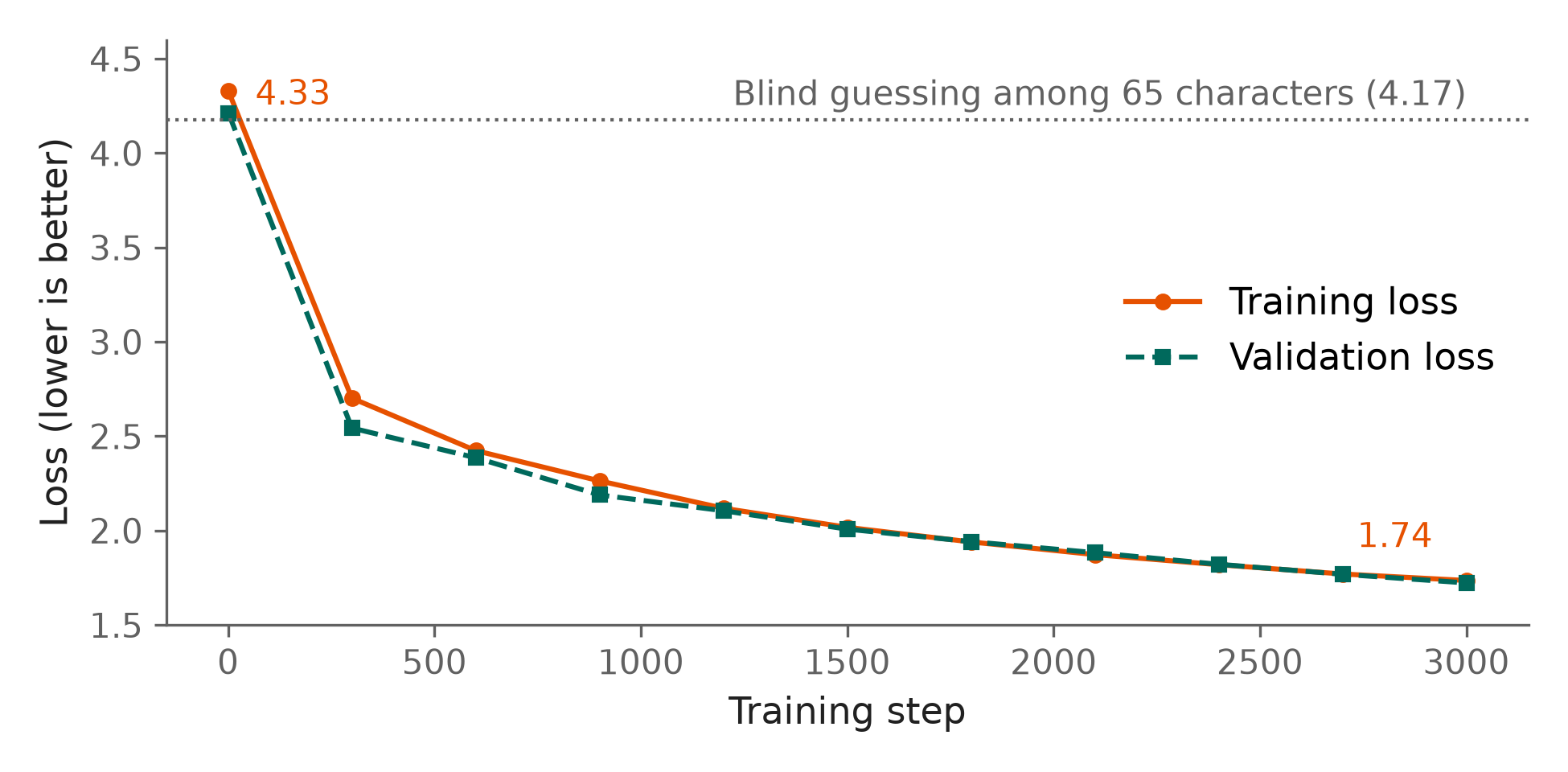Training loss dropping over time Figure 13.4: Over 3,000 steps, the model goes from blind guessing to predicting text with high confidence.

The loss plummets (Figure 13.4). By step 300 it is already at 2.7, and by step 3,000 it reaches 1.74.

What the Loss Number Actually Means¶

A loss of 1.74 means nothing on its own. Here is how to read it.

Cross-entropy is built from one number, the probability the model gave to the character that actually came next. The loss is the negative logarithm of that probability, so undoing the logarithm brings the probability back, and a probability is a number you can reason about:

src/examples/ch13_loss_meaning.py
for name, loss in [("random guessing", math.log(VOCAB)),
                   ("step 1", 4.3280),
                   ("step 300", 2.7016),
                   ("step 3000", 1.7357)]:
    # Cross-entropy is the negative log of the probability given to the right answer
    prob = math.exp(-loss)
    print(f"{name:<16} loss {loss:.2f} -> {prob:6.1%} on the right character")

Terminal

$ python src/examples/ch13_loss_meaning.py
random guessing  loss 4.17 ->   1.5% on the right character
step 1           loss 4.33 ->   1.3% on the right character
step 300         loss 2.70 ->   6.7% on the right character
step 3000        loss 1.74 ->  17.6% on the right character

Now the numbers say something. At the start the model puts about 1.3% of its confidence on the correct character, slightly worse than the 1.5% you would get by drawing at random from 65 characters. Twelve times better than chance by the end sounds impressive, and it is. But read the absolute figure too. Even fully trained, the model is wrong about the next character roughly four times in five.

Hold on to that, because it sets the right expectation for what you built. The model has learned which characters tend to follow which, how long words usually run, where the line breaks fall, and what a speaker's name looks like. It has not learned the rules of English, and it has certainly not learned to mean anything. You will see the evidence in Chapter 17, when it writes "Praviour soul to shall that that are the and not,". The shape of Shakespeare is there, and the sense is not.

The "Training" loop on our map is now complete, and our model is a working engine that has learned the character patterns of its training data.

Code¶

The core loop is simple to write in PyTorch.

src/ch12_train.py (excerpt)
    optimizer = torch.optim.Adam(model.parameters(), lr=train_cfg.learning_rate)

    for step in range(1, train_cfg.max_iters + 1):
        x, y, train_iter = get_batch(train_loader, train_iter, device)

        # Forward pass
        logits = model(x)
        loss = F.cross_entropy(logits.view(-1, gpt_cfg.vocab_size), y.view(-1))

        # Backward pass
        optimizer.zero_grad()
        loss.backward()
        optimizer.step()

Run the full script to watch the loss fall:

Terminal

$ python src/ch12_train.py
Chapter 13: The Training Loop

Model parameters: 824,832
Training on     : cpu
Steps           : 3,000
Batch size      : 32
Block size      : 128

Starting training... (eval every 300 steps)
step     1/3000 | train loss: 4.3280 | val loss: 4.2114 | elapsed: 3s | ETA: 7595s
step   300/3000 | train loss: 2.7016 | val loss: 2.5433 | elapsed: 55s | ETA: 496s
...
step   900/3000 | train loss: 2.2633 | val loss: 2.1889 | elapsed: 160s | ETA: 372s
step  1200/3000 | train loss: 2.1185 | val loss: 2.1053 | elapsed: 210s | ETA: 314s
step  1500/3000 | train loss: 2.0174 | val loss: 2.0078 | elapsed: 248s | ETA: 248s

What just happened:

Line 1 creates an Adam optimizer to handle the weight updates.
Line 3 runs 3,000 steps of training. The log above reached the halfway point after 248 seconds, so the whole run took about eight minutes on the machine that produced it. On the author's 2020 laptop (see the Preface) the same run took about 20 to 30 minutes.
Lines 11 to 13 calculate the gradients and update the weights, driving the training loss down from 4.33 to 1.74. The log prints two losses. The train loss is measured on text the model practices on, and the val loss on the held-out text from Chapter 4.
We saved our hard-earned weights to a file so we can load them later.

Shape Check:

Table 13.1 lists the parameter count.

Table 13.1: Total adjustable parameters in the language model.

Variable	Shape	Meaning
`model.parameters()`	`824,832`	The total number of individual numbers (weights) the optimizer is adjusting.

Try It¶

We can see the mechanics of PyTorch's automatic gradients on a tiny scale.

src/examples/ch13_autograd_demo.py
"""Show how PyTorch automatically calculates gradients to update a weight."""
import torch

# A single weight starting at 2.0
weight = torch.tensor([2.0], requires_grad=True)

# Our simple 'model' multiplies input by weight
x = torch.tensor([3.0])
target = torch.tensor([12.0]) # We want output to be 12

print(f"Initial weight: {weight.item():.2f}")

for step in range(3):
    # Forward pass
    output = weight * x
    loss = (output - target) ** 2

    # Backward pass (calculate the gradient)
    loss.backward()

    print(f"Step {step+1}: Output={output.item():.2f}, "
          f"Loss={loss.item():.2f}, Gradient={weight.grad.item():.2f}")

    # Update weight (move in opposite direction of gradient)
    with torch.no_grad():
        weight -= 0.05 * weight.grad
        weight.grad.zero_()

print(f"Final weight: {weight.item():.2f}")

Lines 19, 26, and 27 show PyTorch computing the gradient and using it to adjust the weight toward the target.

Terminal

$ python src/examples/ch13_autograd_demo.py
Initial weight: 2.00
Step 1: Output=6.00, Loss=36.00, Gradient=-36.00
Step 2: Output=11.40, Loss=0.36, Gradient=-3.60
Step 3: Output=11.94, Loss=0.00, Gradient=-0.36
Final weight: 4.00

Try It

Open src/examples/ch13_autograd_demo.py. Change the starting weight to 10.0 and watch how the gradient pulls it down instead of pushing it up, always aiming for the target output of 12.

In Business

Training is where the real investment happens. When your company trains its house-style assistant, it pays for the compute time required to run this loop billions of times across thousands of documents. The loss curve is your main dashboard metric, because as long as it is going down, the assistant is getting better at mimicking your corporate voice.

Watch Out

Never forget optimizer.zero_grad() before loss.backward(). PyTorch accumulates gradients by default (adds them up). If you don't zero them out at the start of the backward pass, your model will take steps based on a mix of the current batch and all previous batches, wandering off in the wrong direction.

Key Takeaways¶

Training is a loop of four steps: Forward, Loss, Backward, Step.
Gradient descent finds the lowest loss by taking small steps downhill.
We use the torch.optim.Adam optimizer to manage the complex math of updating the weights.
The model starts by guessing blindly (loss > 4.17), but over 3,000 steps, it learns the patterns of the text and the loss plummets.

Check Your Understanding¶

What are the four main steps inside the training loop?
What does loss.backward() actually do?
Why is a dropping loss curve a good sign?

Assignment¶

Assignment 13: Shrink the step

About 15 minutes. You change one number and write no new code. Work in this chapter's Colab notebook or on your own laptop.

Run it. Run src/examples/ch13_autograd_demo.py as it is. Copy the five lines it prints: the initial weight, the three steps and the final weight.
Change one number. Find the line weight -= 0.05 * weight.grad. The 0.05 is the learning rate: how far the weight moves on each step. Change 0.05 to 0.0003 and run the script again.
Compare. Which printed lines are the same in both runs? After three steps, how close does the output get to the target of 12 in each run? Is the loss still falling in the second run?
Explain it. In two or three sentences a manager could follow, say what a learning rate that is too small for the job costs a company that pays for every training step.

Hand in: both sets of five lines, your answers to step 3, and your sentences.

Chapter 13: The Training Loop¶

Theory¶

Walking Down the Hill¶

The Four-Step Loop¶

How Big Should the Step Be?¶

The "Aha!" Moment: It Learned¶

What the Loss Number Actually Means¶

Code¶

Try It¶

Key Takeaways¶

Check Your Understanding¶

Assignment¶

Further Reading¶