The Whole Book on One Page¶

Name: Building an LLM from Zero: Look Inside the Black Box
Author: Truong (Jack) Luu

Every chapter, in order, in one scroll. This edition is here for the things a chapter page cannot do: searching the whole book with your browser's own find, printing it, or reading it straight through without clicking. Use the contents on the left to jump to any chapter or section.

It is a long page, carrying all 75 figures, so give it a moment on a slow connection. The ordinary way to read the book is chapter by chapter, starting at the preface, and there is also a PDF and an EPUB.

First draft: December 17, 2025. Last updated: September 2026.

Preface: Why This Book Exists¶

There are already a lot of resources out there for learning about AI and large language models. So why write another one?

Because most of them fall into one of three traps, or they push you straight into tutorial hell.

Tutorial hell is a state of learning paralysis where you endlessly watch coding tutorials and follow along with instructors, feeling productive, but never actually building anything on your own. You run the code, it works, you feel good, but close the laptop and ask yourself why any of it worked, and you draw a blank. You've watched the chef cook a hundred times but have never touched the stove yourself.

The three traps that lead there:

Too shallow. Copy-and-paste the code, follow along, done. You produce an output, but you don't understand any of the decisions behind it. The moment something breaks or changes, you're stuck.
Too deep. Research-paper density, prerequisite courses in linear algebra and calculus, written for people who already have a graduate-level background. Most readers bounce off in chapter two.
Too demanding on hardware. Great content, but assumes you have a modern GPU, a cloud computing account, and several dedicated weekends free. That rules out most people.

This book is a different approach.

The goal is a balance between theory and code, enough explanation to genuinely understand what you are building and why each piece is there, paired with real, runnable code you can execute right now on the machine in front of you.

Every chapter follows the same structure: first the idea in plain language with an analogy, then the code that implements it, then a short summary. You are never asked to accept something on faith. If a line of code does something, the chapter explains why.

Right now means on a regular laptop. No GPU. No cloud. No special hardware. This entire book was written and tested on a ThinkPad T14 Gen 1 (Intel Core i7, 32 GB RAM, released 2020), a five-year-old business laptop with no dedicated GPU. The full training run completed in about 20-30 minutes. If it runs there, it will run on yours.

Setup is minimal: Python and PyTorch. That's it. No accounts to create, no clusters to configure.

Who Is This Book For?¶

Beginners who learn by building. You know some Python, you're curious about AI, and you want to actually understand how it works, not just use someone else's model. You want to go from zero to a working language model, line by line, without getting stuck in tutorial hell.

Instructors and professors. You want classroom-ready material: concepts clear enough to teach, code that runs on a student's laptop in a single class session, and a structure that maps cleanly to a lecture. This book is designed to be that.

IT/IS professionals. You work with AI tools every day but want to understand what's happening under the hood. You don't need a PhD, you need a clear explanation of the architecture, a working example, and code you can actually read and modify.

Parents teaching their kids. AI is everywhere. If you want to introduce your child to how it actually works, not just how to use it, this book gives you a concrete, hands-on project you can work through together. Build something real. Ask questions. Break it and fix it. That's how learning sticks.

A Note on AI Assistance¶

This book was written by Truong (Jack) Luu. AI tools helped with writing plans, code drafts, and editing. All code was reviewed, edited, and tested by the author on a local machine. Every example in this book runs exactly as shown.

Truong (Jack) Luu jackluu.io

Introduction: Five Phases, One Loop¶

Before you write a line of code, it helps to know where the thing you are about to build sits. Artificial intelligence is not one invention. It is five waves, each of which kept what worked and changed one idea. The model in this book belongs to the fourth wave, and it inherits almost everything from the second.

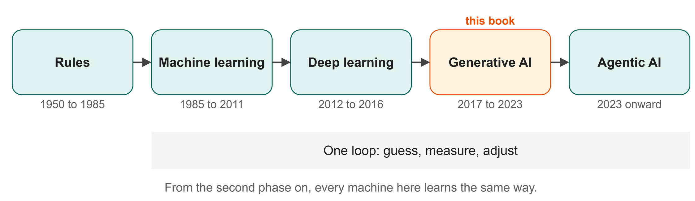The five phases of artificial intelligence on a timeline Figure I.1: Five waves of artificial intelligence. From the second wave onward, every one of them learns the same way.

Where this book sits¶

The first phase, roughly 1950 to 1985, had people write down every rule by hand. If this, then that, thousands of times over. ELIZA, released in 1966, imitated a therapist by spotting a keyword in your sentence and turning it back into a question. It knew nothing, and people confided in it anyway. That is the oldest lesson in the field: we read understanding into anything that answers in fluent sentences.

The second phase, roughly 1985 to 2011, gave up on writing the rule. Show the machine ten thousand emails already labeled spam or not spam, and let it find the pattern itself. This is where the arithmetic of this book begins: turn everything into numbers, guess, measure how wrong the guess was, and nudge the numbers. Nothing since has changed that.

The third phase, 2012 to 2016, changed the scale and nothing else. Stack more layers, use far more data, run it on graphics cards. The result that settled the argument was an image model in 2012 that won its competition by a margin nobody could dispute, using the same loop.

The fourth phase, 2017 to 2023, changed the goal. Earlier models sorted an input into a category. These produce the next piece of it. Two ideas made that work: give every word a position in a space of numbers so that similar words sit near each other, and let the model weigh how much every other word matters before it commits to the next one. That second idea arrived in 2017 and is called attention. The rest of this book is those two ideas, built small enough to read.

The fifth phase, 2023 onward, barely changed the model at all. What changed is what we let it do: give it a goal and a set of tools, and let it plan a step, use a tool, check the result, and plan the next one. The engine underneath is still a next-word predictor. It is the one you are about to build.

Table I.1: The five phases, and what actually changed at each one.

Phase	Roughly	What changed	What the machine does
Rules	1950 to 1985	People write every rule	Matches patterns, follows conditions
Machine learning	1985 to 2011	Learn the rule from examples	Guess, measure the error, adjust
Deep learning	2012 to 2016	Far more layers and data	The same loop, much bigger
Generative AI	2017 to 2023	Produce the next piece, not a label	Embeddings and attention, same loop
Agentic AI	2023 onward	Give the model tools and a goal	The same model, inside a system

One loop, running for forty years¶

Strip away the vocabulary and every phase from the second onward runs the same three steps.

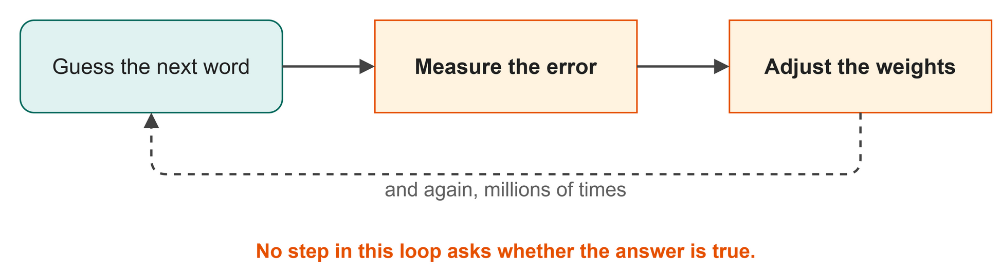The training loop: guess, measure the error, adjust the weights Figure I.2: The loop that every model in this book runs, millions of times.

The machine guesses. Something measures how far the guess landed from the right answer. Something else adjusts the numbers so the next guess lands closer. Then it does it again, millions of times. You will build all three parts: the guess in Chapter 10, the measurement in Chapter 11, and the adjustment in Chapter 13.

Read that loop again and notice what is missing. No step in it asks whether the answer is true. The model is rewarded for producing text that fits the pattern of its training data, and a convincing invention fits that pattern exactly as well as a fact does. This is why language models state false things in clean, confident prose. It is not a defect that better engineering will remove. It is what the loop optimizes for, and you will see it directly in Chapter 17 when your own model writes Shakespeare that no one ever wrote.

A layer is a stack of small regressions¶

If you have fitted a line through a scatter plot, you have already trained a model. You picked a slope and an intercept, measured how far each point missed the line, and chose the values that made the misses smallest. That is the whole idea: a guess, a ruler, an adjustment.

A neural network is that, repeated. Each unit inside a layer multiplies its inputs by its own weights, adds them up, and adds one more number to shift the result. A slope for every input and an intercept, which is a regression. A layer runs a few hundred of those at once, as a single multiplication of two tables of numbers, and a network stacks the layers. Nothing in this book is harder than that; there is only a great deal of it. Chapter 3 covers the tables of numbers, and Chapter 8 builds the layer.

The four parts you are about to build¶

Follow one guess from a chatbot and you pass through four pieces, in this order.

The dictionary. Words are turned into lists of numbers, positioned so that words used alike sit near each other. This is the embedding, and it is Chapter 5.
The structure. Layers of numbers, each doing its small job and handing the result to the next. Attention lives here, in Chapters 6 through 10.
The ruler. A single number saying how far the guess landed from the right answer. This is the loss, and it is Chapter 11.
The messenger. The error is carried back through every layer, telling each weight which way to move. This is backpropagation, and it runs the training in Chapter 13.

Why build it by hand¶

A calculator is a fine thing if you already know arithmetic. If you never learned it, you will not notice when the calculator gives you a wrong answer, because you have nothing to check it against.

That is the argument for this book. You can already get a language model to write code, draft a memo, or explain itself. What you cannot do, without having built one, is tell when it is wrong, and say why. By the end you will have written every part of a working model, trained it on your own laptop, watched its error fall, and read the text it produces. After that, the polished paragraph on your screen stops being magic and becomes a machine you understand well enough to doubt.

Module 1: Foundations¶

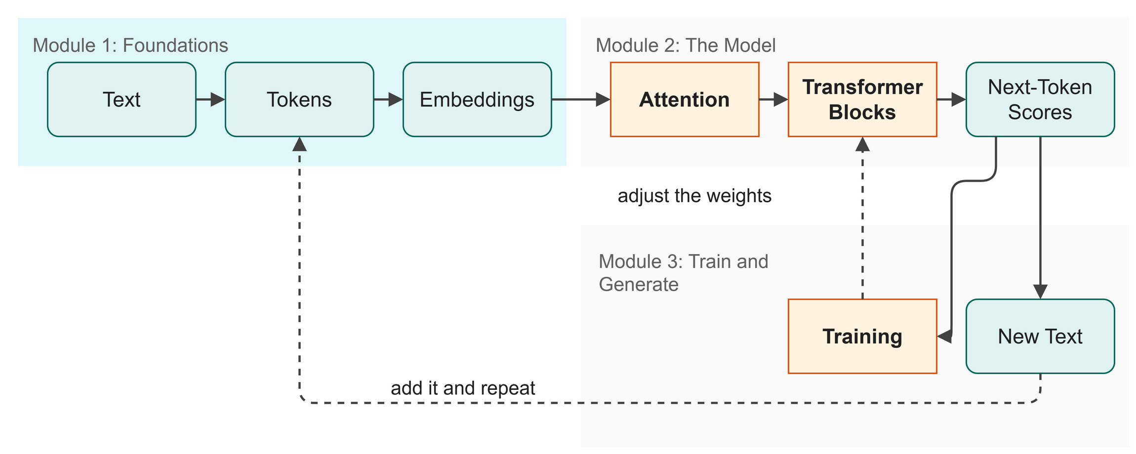Module 1 Map Figure M1.1: Foundations in the big picture.

In this first module, we set up our workspace and prepare the raw material for our language model. For business readers, imagine you are building an assistant to draft text in your company's house style, trained on the company's archive. Think of this module as data preparation: before any system can find patterns, the text must be translated into numbers it can process.

In this module you will:

Set up Python and PyTorch on your computer
Understand what a language model actually does
Learn how tensors work as the foundation for our math
Build a tokenizer to chop text into manageable pieces
Create embeddings that give those pieces mathematical meaning

Chapter 1: Environment Setup¶

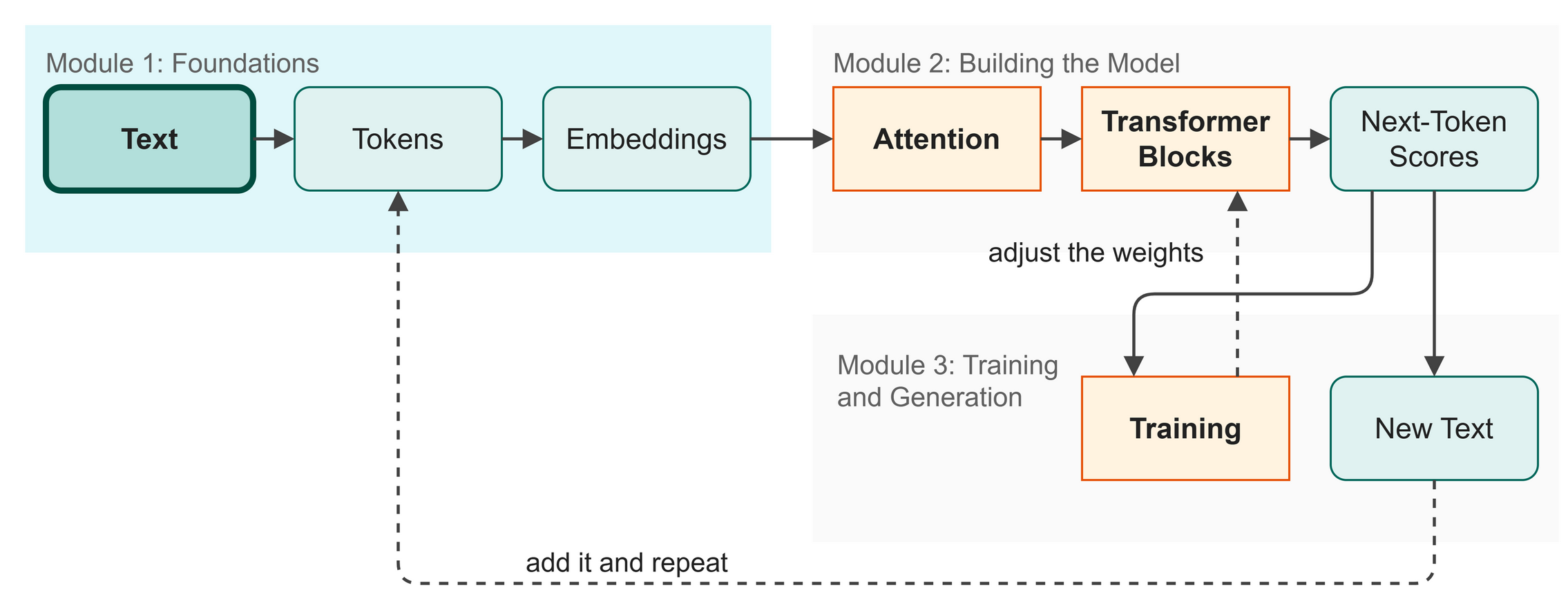The map highlights the environment setup stage Figure 1.1: Before you build, you set up your tools.

Setting up your environment ensures you have all the tools needed to build and run the model (as shown in Figure 1.1). This creates a predictable foundation so the code works the same way for you as it does in this book.

In this chapter you will:

Install Python and a terminal to run commands.
Download the project code using Git.
Set up an isolated workspace for your packages.
Download the training dataset.

Words to Know

Terminal: a text-based window where you type commands.
Repository: a folder of code stored online.
Virtual Environment: an isolated toolbox for a single project's packages.
Package Manager: a tool that downloads and installs code libraries.

In Business

Standardizing development environments in tech teams prevents the classic "it works on my machine" problem. When a company builds a house-style AI assistant to draft emails, the development team standardizes their environment. By using virtual environments and fixed package versions, companies ensure that new hires can start working immediately on the AI assistant and code runs identically on laptops and production servers.

Step 1: Install Python¶

Python is the programming language this entire tutorial uses. We need version 3.10 or newer. As seen in Figure 1.2, you can download it from the official website.

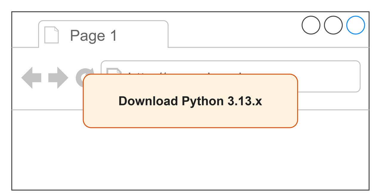A generic browser window showing the python.org downloads page with a download button Figure 1.2: Download the latest Python installer.

Windows:

Open your web browser and go to python.org/downloads
Click the button to download Python 3.13.x.
Run the downloaded .exe installer.
CRITICAL: On the first screen of the installer, check the box that says "Add Python to PATH" at the very bottom. If you miss this, Python will not be found when you type commands.
Click "Install Now".

macOS:

Open your web browser and go to python.org/downloads
Click the button to download Python 3.13.x.
Run the downloaded .pkg installer and follow the prompts.

Step 2: Open a Terminal¶

The terminal is where you will run your code.

Windows: Press Win + R, type cmd, and press Enter. A black window appears with a blinking cursor.

macOS: Press Cmd + Space to open Spotlight, type Terminal, and press Enter.

Verify your Python installation by running this command:

Terminal

$ python --version

You should see Python 3.10 or newer printed to the screen. (On macOS, if python is not found, type python3 --version instead.)

Step 3: Install Git¶

Git downloads the project code from the internet. Figure 1.3 shows the download page.

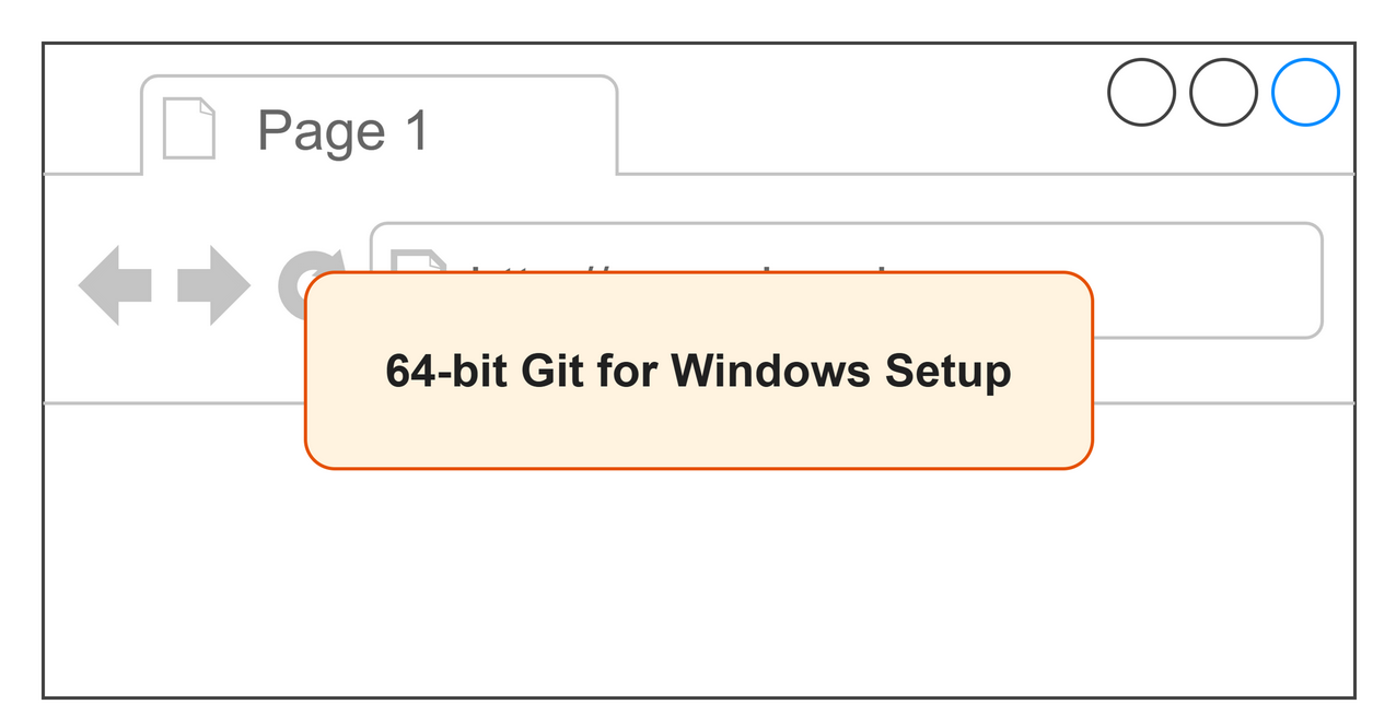A generic browser window showing the Git download page Figure 1.3: Download Git to get the project files.

Windows:

Go to git-scm.com/download/win
Download the "64-bit Git for Windows Setup".
Run the installer and click "Next" through every screen.

macOS: Open your terminal and type git --version. If it is not installed, macOS will ask if you want to install the "Command Line Developer Tools". Click Install.

Verify Git is installed (open a new terminal window on Windows):

Terminal

$ git --version

You should see a message confirming your Git version.

Step 4: Download the Project¶

Now download the project code with a single command.

Terminal

$ git clone https://github.com/jackluucoding/build-llm-from-zero.git

Then move into the project folder:

Terminal

$ cd build-llm-from-zero

Step 5: Create a Virtual Environment¶

Different projects need different versions of the same library. A virtual environment gives this project its own isolated box of packages. Figure 1.4 illustrates this isolation.

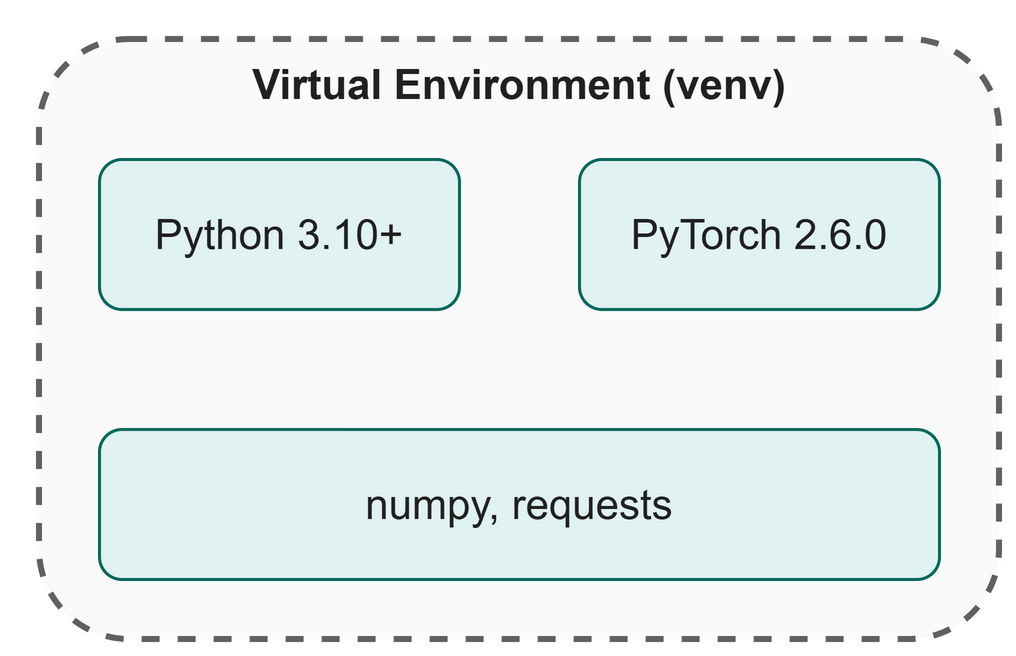A dashed box representing a virtual environment containing Python and PyTorch Figure 1.4: A virtual environment isolates your project's libraries.

Make sure your terminal is inside the build-llm-from-zero folder, then run:

Windows:

Terminal

$ python -m venv venv
$ venv\Scripts\activate

macOS:

Terminal

$ python3 -m venv venv
$ source venv/bin/activate

You will see (venv) appear at the start of your terminal prompt. You must run the activate command every time you open a new terminal window.

Step 6: Install PyTorch and Dependencies¶

With the virtual environment active, install the required libraries using pip, Python's package manager.

First, install PyTorch (we use a CPU-only version):

Terminal

$ pip install torch==2.6.0 --index-url https://download.pytorch.org/whl/cpu

Then install the other libraries:

Terminal

$ pip install numpy requests matplotlib

Step 7: Download the Shakespeare Dataset¶

We will train our model to write in a specific style using the complete works of Shakespeare. (Dataset credit: the Tiny Shakespeare text comes from Andrej Karpathy's char-rnn project, https://github.com/karpathy/char-rnn)

Terminal

$ python src/utils/download_data.py
Dataset statistics:
  Total characters : 1,115,394
  Unique characters: 65

First 200 characters:

Step 8: Verify Everything Works¶

Run the setup verification script to confirm all pieces are ready:

Terminal

$ python src/ch00_setup_check.py
Chapter 1: Checking your environment...

[OK] Python: 3.13.13
[OK] PyTorch: 2.6.0+cpu
[OK] NumPy: 2.5.3
[OK] Requests: 2.34.2
[OK] Shakespeare dataset found: 1,115,394 characters
[OK] Quick tensor test passed

All checks passed! You are ready to start Chapter 1.

If you see this, you are fully ready to begin!

Watch Out

If a script fails with ModuleNotFoundError: No module named 'torch', your virtual environment is not active. Run the activate command again (venv\Scripts\activate on Windows, source venv/bin/activate on macOS).

Key Takeaways¶

You installed Python (the language), Git (code downloader), PyTorch (math library), and a terminal.
A virtual environment keeps this project's packages isolated.
Always activate your virtual environment before working on this project.
With your environment ready, you can now move on to the next step in our map.

Check Your Understanding¶

What does a virtual environment do?
How do you know if your virtual environment is active?
What is the command to move into the project folder?

Chapter 2: What Is an LLM?¶

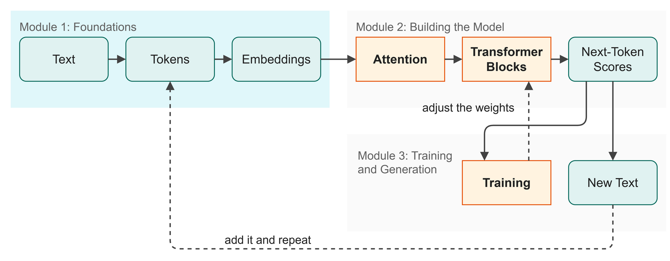The map highlights the whole chain as an overview Figure 2.1: Before we zoom in, let's look at what the whole system actually does.

With our environment set up in the previous chapter, we are ready to understand the model itself (Figure 2.1). A Language Model (LM) seems like a magic box that understands what you type. But under the hood, it performs a very specific, simple task.

In this chapter you will:

Learn the single rule that drives all language models.
See how models generate long answers one step at a time.
Understand how reading data replaces human teachers.

Words to Know

Token: one small piece of text, here a single character.
Language Model: a system that predicts the next token in a sequence.
Autoregressive: using your past outputs as inputs for your next step.
Parameters: the numbers inside the model that adjust during training.

Theory: The Next-Token Engine¶

Imagine you are texting a friend and you type: "I am so hungry, I could eat a". Before you finish, your phone suggests: horse. Or pizza.

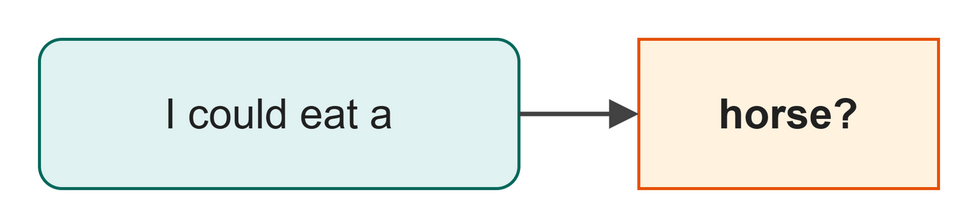A text box with incomplete text points to a prediction box showing horse Figure 2.2: The core task of a language model is guessing what comes next.

As Figure 2.2 shows, your phone is doing next-word prediction. It guesses what word is most likely to come next based on everything you typed so far. A Large Language Model (LLM) does exactly the same thing. Given a sequence of tokens, it predicts what comes next. That is the whole idea. Everything else in this book is just building a machine that can do this really well.

How It Talks Back¶

If the model only predicts the next token, how does it write an essay? It uses autoregressive generation.

You type: "What is the capital of France?"
The model predicts the next token: "Paris".
That output is added to the input: "What is the capital of France? Paris".
It predicts the next token: " is".
And repeats until it decides to stop.

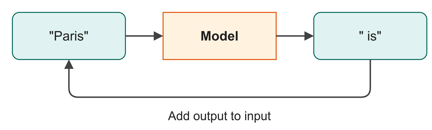A diagram showing the output text being fed back into the model as input Figure 2.3: In autoregressive generation, each predicted output loops back to become the next input.

As illustrated in Figure 2.3, the model never thinks about the whole answer at once. It just keeps predicting the next piece, over and over, building the sentence step by step.

What is a Token?¶

A token is the smallest unit the model works with. It could be a whole word, a piece of a word, or just a single character.

In this book, we use character-level tokens. Every single letter, space, and punctuation mark is one token. We use characters because the vocabulary is tiny (only 65 characters in our Shakespeare data) and you can understand it instantly. Real models use more complex chunks (subwords), but the math is exactly the same.

The Power of Self-Supervised Learning¶

To make a model "Large", we give it millions of parameters, which are the numbers inside the model that act like dials. Training turns these dials until the model produces good output.

But how does it learn without a teacher grading its work? Through self-supervised learning.

With language, the text itself is the answer key. If your training text is "Hello world", the model gets these practice questions automatically:

See H, predict e.
See He, predict l.
See Hel, predict l.

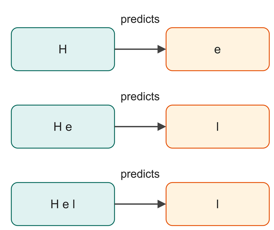A diagram showing text subsets predicting the next character Figure 2.4: The text itself provides thousands of built-in practice questions.

As Figure 2.4 demonstrates, because no human labels are needed, you can train a model on millions of pages of raw text. The model just reads the data and learns the patterns.

Try It: The Numbers Game¶

Is it really just predicting characters? Let's prove it by looking at real data. If we see the letters "the ", what is the most likely next character in Shakespeare?

We wrote a tiny script to scan our training data and count every character that follows "the ".

Terminal

$ python src/examples/ch02_next_char.py
What follows 'the ' in Shakespeare?
's': 573 times
'w': 459 times
'c': 448 times
'p': 426 times
'm': 376 times

This is exactly what the model learns to do, but instead of counting by hand, it uses math to predict the probabilities.

In Business

If a company builds an AI assistant to draft emails in its own house style, the concept is the same. The model trains on the company's archive of past writing. By learning what character or word typically follows another in that specific archive, the assistant learns the company's unique voice and terminology automatically.

Watch Out

It is easy to think the model "understands" the text. It does not. It is simply a math engine calculating the most probable next token based on patterns in its training data.

Key Takeaways¶

A language model is a system that predicts the next token.
Autoregressive generation means the model uses its own outputs as inputs for the next step.
Tokens are the basic pieces of text, like characters or words.
Self-supervised learning uses the raw text itself as the answer key.
Now that we know the whole system revolves around next-token prediction, let's zoom in on the first step in our map: the math and tools we use to build it.

Check Your Understanding¶

What does a language model actually predict?
Why is it called "autoregressive"?
How does self-supervised learning differ from having a teacher grade the work?

Chapter 3: Tensors and PyTorch¶

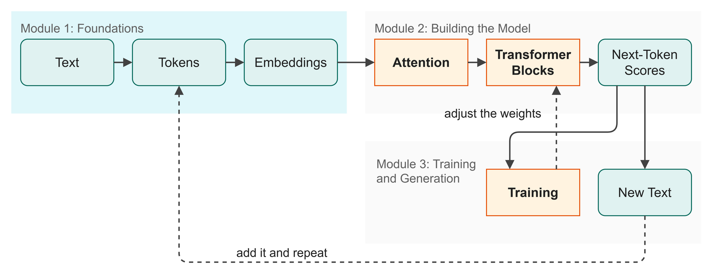The map highlights the whole chain, as tensors are the foundation for everything Figure 3.1: Tensors are the containers that carry data through every stage.

Now that we understand the language model's goal from the previous chapter, we are ready to start building (Figure 3.1). Before we turn text into numbers, we need a way to store and manipulate those numbers efficiently. Tensors are the specialized containers that do this job, and PyTorch is the engine that processes them. (Note: the exact numbers you see may differ slightly on your computer or PyTorch version).

In this chapter you will:

Learn what a tensor is and how it stores data.
See how tensor shapes represent different dimensions.
Understand how matrix multiplication transforms data.
Turn raw scores into probabilities using Softmax.

Words to Know

PyTorch: a library for doing math on large arrays of numbers very quickly.
Tensor: a multi-dimensional array of numbers.
Shape: the dimensions of a tensor (like rows and columns).
Matrix Multiplication: combining two tensors to transform data.
Softmax: a function that turns any numbers into probabilities that sum to 1.

Theory: The Data Containers¶

PyTorch is a Python library for doing math on large arrays of numbers, really, really fast. Without PyTorch, training would take weeks instead of minutes because pure Python is too slow for millions of calculations.

A 1D vector, a 2D matrix, and a 3D tensor shown as shapes Figure 3.2: Tensors can be 1D (a list), 2D (a table), or 3D (a stack of tables).

A tensor is just a multi-dimensional array of numbers (Figure 3.2). If you have ever used a spreadsheet, you already know 2D tensors. A 3D tensor is just a stack of spreadsheets.

In this book, we work mostly with 3D tensors. Their dimensions, or shape, represent:

B = Batch size (how many sequences we process at once)
T = Time (how many tokens in each sequence)
C = Channel size (how many numbers we use to represent each token)

We write shapes like (B, T, C). For example, (32, 128, 128) means "32 sequences, each 128 tokens long, each token described by 128 numbers."

Matrix Multiplication as Data Transformation¶

A data tensor and a transformation tensor combine to make a result tensor Figure 3.3: Matrix multiplication transforms data from one shape to another.

Matrix multiplication (written as @ in Python) is how neural networks transform data, as shown in Figure 3.3. The rule is that the inner dimensions must match: a (3, 4) tensor can multiply a (4, 5) tensor, creating a new (3, 5) tensor.

Think of (3, 4) as "3 students each with 4 test scores" and (4, 5) as "4 test scores each mapped to 5 skill ratings". Multiplying them gives you "3 students each with 5 skill ratings".

Softmax: Turning Scores into Probabilities¶

As Figure 3.4 shows, Softmax is a mathematical function that takes any list of numbers (called logits) and turns them into probabilities. The probabilities are all positive and always sum to exactly 1.0. It does this using exponential functions, which make the highest numbers stand out even more.

A diagram showing raw scores 1.0, 2.0, 3.0 turning into probabilities 0.09, 0.24, 0.67 Figure 3.4: Softmax forces numbers into a 0-to-1 range where they total exactly 1.0.

Code: Basic Operations¶

Let's look at the basic PyTorch operations we will use.

src/ch02_tensors.py (excerpt)
    # A 1D tensor is simply a list of numbers
    a = torch.tensor([1.0, 2.0, 3.0, 4.0])

    # A 2D tensor represents a table or matrix of numbers
    b = torch.tensor([[1.0, 2.0, 3.0], [4.0, 5.0, 6.0]])

    x = torch.randn(2, 5, 8)
    W = torch.randn(8, 4)
    y = x @ W

Run the file to see how PyTorch handles these:

Terminal

$ python src/ch02_tensors.py
--- 1. Creating tensors ---
1D tensor: tensor([1., 2., 3., 4.])
  shape: torch.Size([4])
...

...
        [ 0.2303, -1.1229, -0.1863]])
...
tensor([[ 0.,  1.,  2.,  3.],
...

...

What just happened:

Lines 2 and 5 created 1D and 2D tensors, printing their shapes.
Line 7 looked at a 3D tensor with a shape of (2, 5, 8), representing (Batch, Time, Channels).
Line 9 multiplied a 3D tensor by a 2D matrix. PyTorch automatically applied the multiplication across the batch dimension. This is called batched matrix multiplication, and it saves us from writing slow Python loops.

Shape Check

Table 3.1 shows the tensor shapes before and after matrix multiplication.

Table 3.1: Tensor shapes before and after matrix multiplication.

Tensor	Shape	Meaning
`x`	`(2, 5, 8)`	2 sequences, 5 tokens each, 8 numbers per token
`W`	`(8, 4)`	Transformation weights: 8 inputs to 4 outputs
`y`	`(2, 5, 4)`	2 sequences, 5 tokens each, now 4 numbers per token

Try It

Open src/ch02_tensors.py, change logits = torch.tensor([1.0, 2.0, 3.0]) to [1.0, 2.0, 10.0], and run it. Notice how the highest number takes almost 100% of the probability after Softmax.

In Business

How data is represented matters. When building our house-style email assistant, the text data is transformed into multi-dimensional tensors. The math operations we just covered are exactly how the assistant processes massive datasets to find hidden patterns in your company's writing voice.

Watch Out

A shape mismatch is the most common error in PyTorch. If you try to multiply (3, 4) and (5, 6), PyTorch will crash because the inner dimensions (4 and 5) do not match. Always check your shapes!

Key Takeaways¶

A tensor is a multi-dimensional array of numbers.
Shape (B, T, C) = batch × time × channels, the standard convention in this book.
@ is matrix multiplication. Inner dimensions must match.
Softmax turns any numbers into probabilities that sum to 1.
PyTorch handles batches automatically using batched matrix multiplication, with no for-loops needed.
With tensors ready to hold our data, we can move to the next stage in our map: turning text into tokens.

Check Your Understanding¶

What does the shape (32, 128, 128) represent in our (B, T, C) format?
Why do the inner dimensions need to match in matrix multiplication?
What is the difference between logits and probabilities?

Chapter 4: Tokenization¶

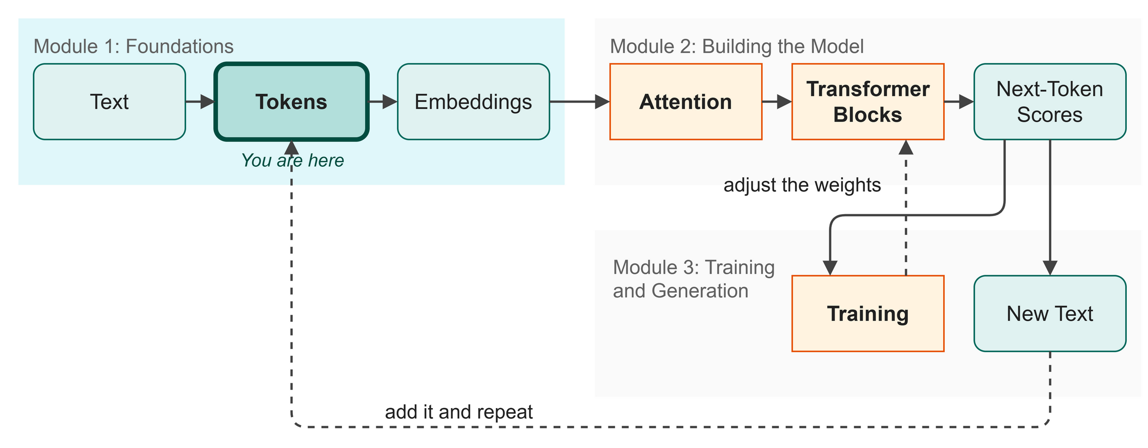Where we are Figure 4.1: Tokenization in the big picture.

Now that we have tensors to hold our data from the previous chapter, we are ready to move to the next stage in our map (Figure 4.1). Before a language model can find patterns in text, we must translate that text into a format it can understand. Neural networks only do math, which means they only eat numbers. In this chapter, we build our tokenizer: a translator that chops text into small pieces and assigns a number to each one.

In this chapter you will:

Understand why neural networks need numbers
Build a character-level vocabulary from the Shakespeare dataset
Write functions to encode text into integers and decode it back
Prepare the data for training by splitting it into two sets

Words to Know

Token: one small piece of text, here a single character.
Tokenizer: a function that turns text into tokens and then into numbers.

Theory¶

Neural Networks Are Number Machines¶

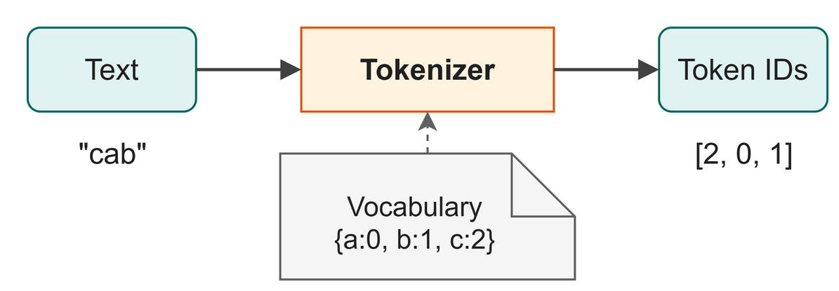Text goes in, numbers come out: each character maps to one ID Figure 4.2: A tokenizer turns each character into a number.

Neural networks cannot read. You cannot feed them a string like "Hello". They expect a grid of numbers to multiply and add. To feed text into a model, we must first convert it into numbers. This process, illustrated in Figure 4.2, is called tokenization.

We need a consistent rulebook. If the letter a is the number 0, it must always be 0. We call this rulebook our vocabulary.

The Simplest Tokenizer¶

There are many ways to tokenize text. You could map each full word to a number (word-level). You could group common letters like th together (subword-level).

For our model, we use the simplest approach: character-level tokenization. Every unique character in our dataset gets its own unique integer. If our vocabulary is just {a: 0, b: 1, c: 2}, then the word "cab" becomes [2, 0, 1].

The Shakespeare dataset contains exactly 65 unique characters. This includes uppercase letters, lowercase letters, spaces, and punctuation. If we give each one an ID from 0 to 64, we can translate any Shakespearean sentence into a list of integers.

In Business

When you build an assistant to draft text in your company's house style, tokenization choices matter. A character-level tokenizer is simple but makes sequences long. A word-level tokenizer makes sequences short but requires a massive vocabulary. Modern business assistants use Byte-Pair Encoding (BPE), a middle ground that groups common character sequences into single tokens. We use character-level here because it keeps the math clean while our model learns from its archive (our Shakespeare dataset).

The Training and Validation Split¶

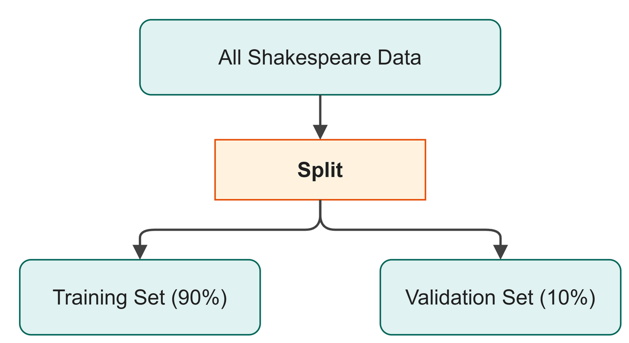Splitting the dataset into training and validation sets Figure 4.3: Hiding part of the data lets us test if the model actually learned.

Once we encode all of Shakespeare into one massive list of numbers, we split it into two piles (Figure 4.3):

Training set (90%): The data the model studies to learn patterns.
Validation set (10%): The data we hide from the model, used to test it later.

Why hide data? We want to know if the model is picking up patterns that hold across the text, or just memorizing the passages it was shown. If it performs well on the training set but fails on the validation set, it is overfitting.

Watch Out

Our tokenizer only knows the characters it saw in the training data. If you feed it a digit (like 1 or 2), an emoji, or a Chinese character, Python will raise a KeyError because that character is not in our 65-character vocabulary.

Code¶

We write our tokenizer in Python, load the dataset, and encode it.

File: src/ch03_tokenizer.py Run it: python src/ch03_tokenizer.py

src/ch03_tokenizer.py (excerpt)
def build_vocab(text):
    # Find all unique characters in the text
    chars = sorted(set(text))

    # Dictionaries to translate between characters and their integer IDs
    char_to_id = {ch: i for i, ch in enumerate(chars)}
    id_to_char = {i: ch for i, ch in enumerate(chars)}

    return chars, char_to_id, id_to_char

Here is what this code does:

Line 3 uses set(text) to find every unique character in the entire text.
Line 3 uses sorted() to put them in alphabetical order so the IDs stay consistent.
Lines 6 and 7 build two dictionaries: one to go from character to ID (char_to_id), and one to go back (id_to_char).

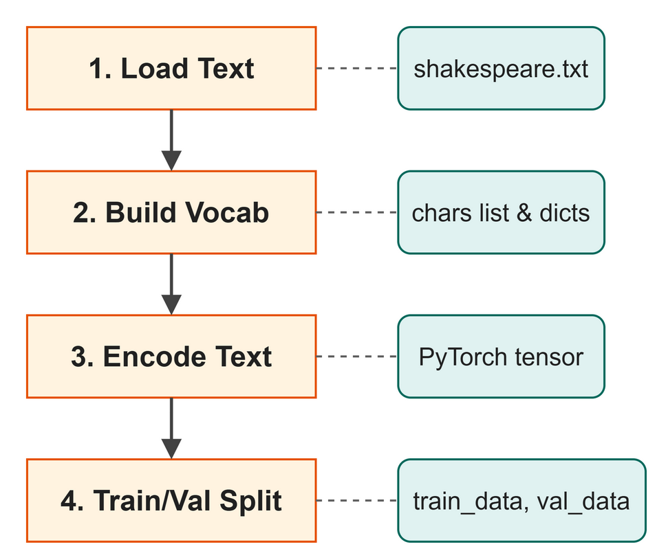Code flow for the tokenizer script Figure 4.4: How the tokenizer processes the dataset.

As Figure 4.4 shows, the script processes the dataset step by step. Next, we write the translation functions:

src/ch03_tokenizer.py (excerpt)
def encode(text, char_to_id):
    # Convert a string into a list of integer IDs
    return [char_to_id[ch] for ch in text]

def decode(ids, id_to_char):
    # Convert a list of integer IDs back into a string
    return "".join([id_to_char[i] for i in ids])

Line 3 converts a string into a list of integer IDs, and line 7 converts them back into a string.

Let's run the script and see what our 65 characters look like, and test a quick round-trip.

Terminal

$ python src/ch03_tokenizer.py
 !$&',-.3:;?ABCDEFGHIJKLMNOPQRSTUVWXYZabcdefghijklmnopqrstuvwxyz
...
--- Testing encode / decode ---
Original : 'Hello, World!'
Encoded  : [20, 43, 50, 50, 53, 6, 1, 35, 53, 56, 50, 42, 2]
Decoded  : 'Hello, World!'
Round-trip matches: True

--- Encoding the full dataset ---

What just happened:

The script loaded over a million characters from the dataset.
It found exactly 65 unique characters. Notice the space and newline characters at the start!
It translated the string "Hello, World!" into a list of integers.
It translated those integers back to prove no data was lost.

Finally, we encode the entire dataset into a PyTorch tensor and split it.

Terminal

Training tokens  : 1,003,854
Validation tokens: 111,540

Tokenizer ready! Ready for Chapter 5.

Try It¶

See how different inputs are converted into numbers. We wrote a short script that imports our tokenizer and encodes a few business phrases.

Try It

Open the terminal and run the example script. Notice how every letter, space, and punctuation mark is assigned a specific number from our vocabulary.

Terminal

$ python src/examples/ch04_tokenizer_demo.py
Demo: Encoding short business phrases
'invoice'       -> [47, 52, 60, 53, 47, 41, 43]
'URGENT!'       -> [33, 30, 19, 17, 26, 32, 2]
'Hello.'        -> [20, 43, 50, 50, 53, 8]

Key Takeaways¶

Neural networks process numbers, not text.
Tokenization translates text into numbers using a fixed vocabulary.
We use a character-level tokenizer with a vocabulary of 65 characters.
encode() turns strings into lists of IDs; decode() turns IDs back into strings.
We split our data into a training set (to learn) and a validation set (to test).

Check Your Understanding¶

Why must we convert text to numbers before feeding it to a language model?
In our character-level tokenizer, what happens if we try to encode a character that wasn't in the training data?
What is the purpose of the validation set?
How many unique characters are in our vocabulary?

Chapter 5: Embeddings¶

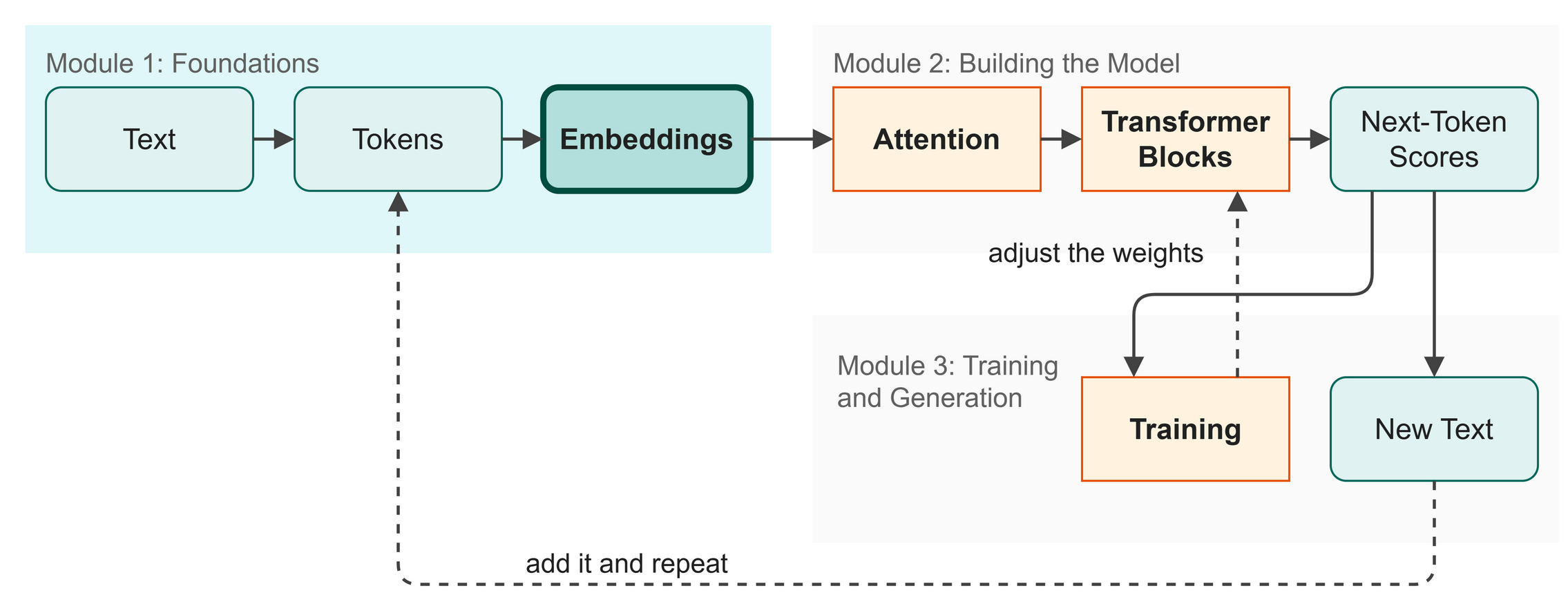Where we are in the big picture Figure 5.1: We have numbers, now we give them meaning.

In the previous chapter, we turned text into tokens (Figure 5.1). Tokens are just arbitrary numbers. To predict what comes next, the model needs to understand how characters relate to each other. In this chapter you will:

Map simple token IDs to large vectors of numbers.
Learn how these vectors capture meaning as coordinates.
Add position information so the model knows the order of characters.

Words to Know

Vector: A list of numbers that acts as a coordinate in a high-dimensional space.
Embedding: A lookup table that maps a token ID to its vector.

Theory¶

The Problem with IDs¶

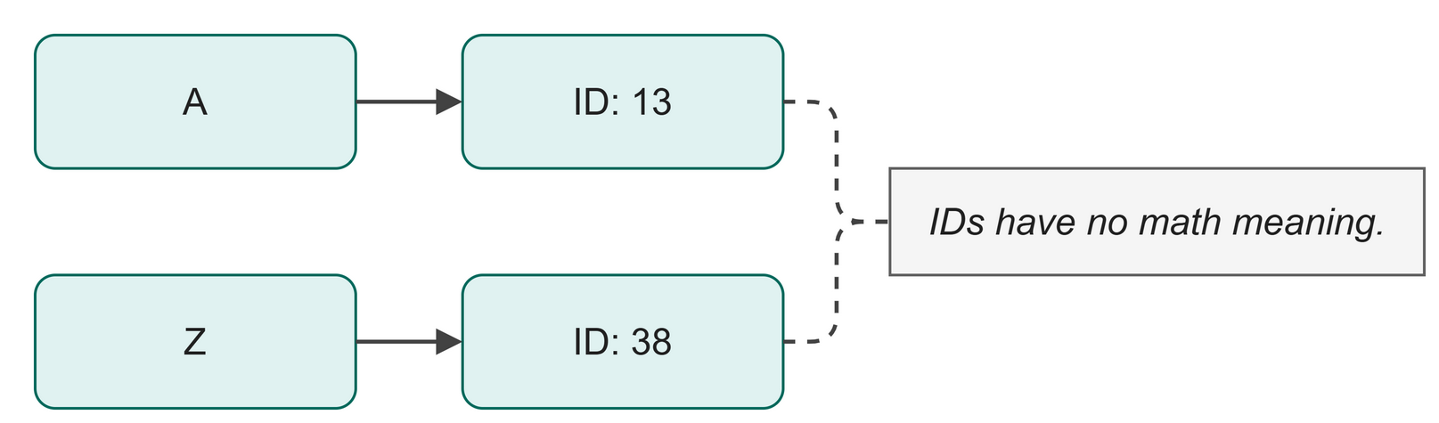IDs have no math meaning Figure 5.2: Token IDs are just arbitrary labels, not math quantities.

After tokenization, each character is an integer: A=13, B=14, a=39. But as Figure 5.2 illustrates, feeding these raw integers to a neural network creates a problem. The network learns by multiplying numbers together. It would see Z (token 38) as almost three times as big as A (token 13). It might learn that Z is more important than A just because of this accident. But token IDs are arbitrary labels.

Think of it like an employee ID number. Employee 105 is not "five times more employee" than Employee 21. The number alone carries no meaning about their role. We need a way to turn these arbitrary labels into a format the "Numbers Machine" can use to find patterns.

Vectors as Coordinates of Meaning¶

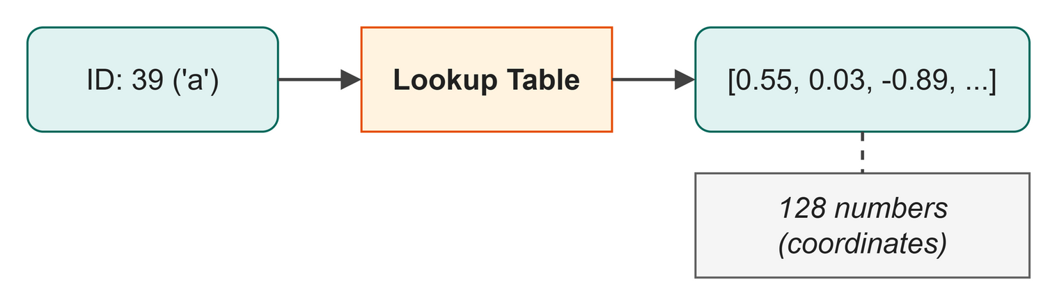Looking up a token ID to find its embedding vector Figure 5.3: An embedding table maps each ID to a vector of numbers.

The solution, shown in Figure 5.3, is a lookup table called an embedding. It maps each token ID to a vector of floating-point numbers. In our model, we use 128 numbers for each character.

Instead of seeing 39 for a, the model sees [0.55, 0.03, -0.89, ...]. These 128 numbers act like coordinates. Characters that appear in similar contexts will gradually be moved closer together in this 128-dimensional space during training. The network learns that capital and lowercase versions of a letter behave similarly, so their vectors become similar. This table of profiles is learned from scratch.

Position Embeddings¶

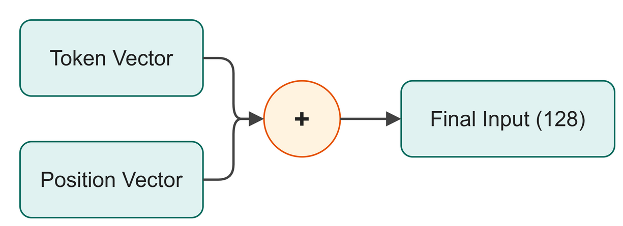Adding token and position embeddings together Figure 5.4: The final representation combines what the token is with where it sits.

There is one more problem: the model reads all characters at exactly the same time. Without help, it cannot tell the difference between "cat" and "act" because they use the same letters. Order matters.

We fix this with positional embeddings (Figure 5.4): a second lookup table indexed by the position of the character in the sequence (0, 1, 2, ...) rather than its token ID. Position 0 gets its own 128-number vector, position 1 gets a different vector, and so on.

We then add the token embedding and the positional embedding together. The network learns to use these combined 128 numbers to represent both "what character is this?" and "where does it appear?". This combined representation completes the "Embeddings" stage in our map (Figure 5.1). The text is now fully converted into rich math vectors, ready for the next stage.

In Business

When you build an assistant that writes in your company's house style, embeddings turn your archive into a landscape of meaning. Token embeddings capture the vocabulary, while the position embeddings give the model the order of the characters, which is what lets it pick up the shape of an invoice or a polite greeting.

Code¶

We use src/ch04_embeddings.py to create and combine these two tables.

src/ch04_embeddings.py (excerpt)
    token_emb = nn.Embedding(config.vocab_size, config.n_embd)
    token_embeddings = token_emb(token_ids)
    pos_emb = nn.Embedding(config.block_size, config.n_embd)
    positions = torch.arange(T)
    position_embeddings = pos_emb(positions)
    x = token_embeddings + position_embeddings

Here is what happens when we run it:

Terminal

$ python src/ch04_embeddings.py
--- 2. Looking up embeddings ---
Input token_ids shape : torch.Size([2, 5])
Token embeddings shape: torch.Size([2, 5, 128])
  (B=2, T=5, C=128)
...
--- 3. Positional embeddings ---
Position indices: [0, 1, 2, 3, 4]
Position embeddings shape: torch.Size([5, 128])

--- 4. Combining token + position embeddings ---
Final x shape: torch.Size([2, 5, 128])
  (B=2, T=5, C=128)

What just happened:

Line 1 created a lookup table for the 65 characters in our vocabulary.
Line 2 translated a batch of token IDs into their embedding vectors.
Line 3 created a second lookup table for the sequence positions.
Line 6 added the token and position vectors to create the final input x.

Shape Check: Table 5.1 details the dimensions of our data structures.

Table 5.1: Tensor shapes before and after the embedding layer.

Variable	Shape	Meaning
`token_ids`	`[B, T]`	Batch size by Time (sequence length).
`token_embeddings`	`[B, T, C]`	`C` is the embedding dimension (128).
`position_embeddings`	`[T, C]`	One vector per position.
`x`	`[B, T, C]`	The combined input for the model.

Try It¶

Try It

Change the batch size B or the sequence length T in src/ch04_embeddings.py. Run the script again. Notice that the output shapes scale automatically, but the parameter counts stay exactly the same. The lookup tables do not care how much text you process at once.

Watch Out

A common mistake is trying to look up a token ID that is larger than the vocabulary size. If your vocab_size is 65, the valid IDs are 0 to 64. Passing an ID of 65 will crash the program with an "index out of bounds" error.

Key Takeaways¶

Token IDs are arbitrary labels and cannot be used directly for math.
Embeddings are learned lookup tables that map token IDs to vectors.
These vectors act as coordinates that capture relationships and meaning.
Positional embeddings are added to tell the model the order of the characters.

Check Your Understanding¶

Why do neural networks struggle with raw token IDs?
How many numbers make up a single character's embedding vector in our model?
Why do we need positional embeddings in addition to token embeddings?
Does the size of the embedding table depend on the batch size?

Module 2: Building the Model¶

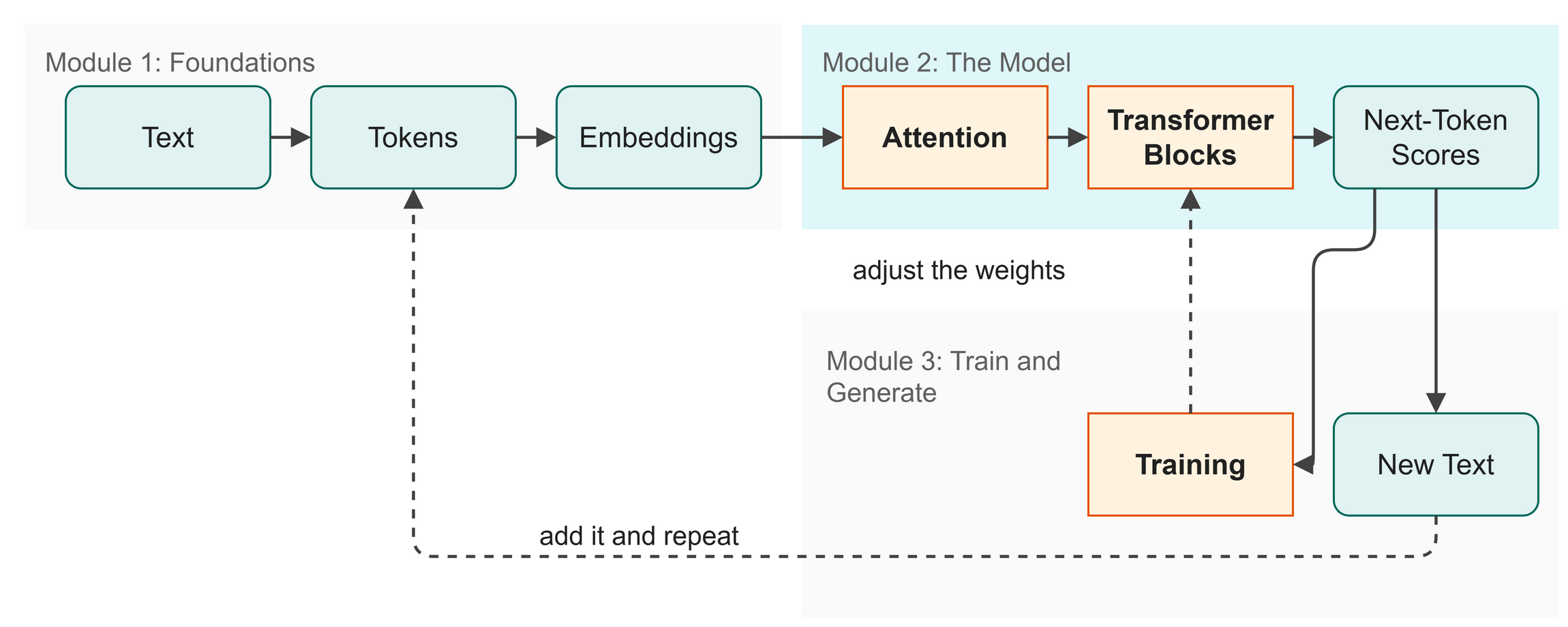Module 2 Map Figure M2.1: Building the Model in the big picture.

Now that we have our data ready, we build the engine. In business terms, this is constructing the logic pipeline that processes information for your house-style writing assistant. We will build the transformer architecture piece by piece, focusing on how attention allows the model to understand context.

In this module you will:

Build self-attention so words can look at each other
Expand to multi-head attention for multiple perspectives
Add feed-forward layers to process what the attention found
Combine these into a complete transformer block
Stack the blocks into the full GPT architecture
Enforce causal language modeling so the model cannot cheat

Chapters¶

Chapter 6: Self-Attention (Single Head)
Chapter 7: Multi-Head Attention
Chapter 8: Feed-Forward and Norms
Chapter 9: The Transformer Block
Chapter 10: The Full GPT Architecture
Chapter 11: Causal Language Modeling

Chapter 6: Self-Attention (Single Head)¶

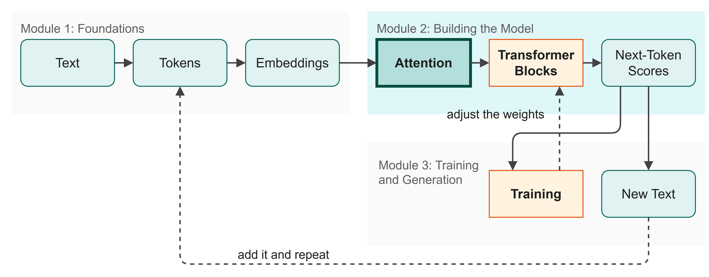Where we are in the big picture Figure 6.1: Attention builds context by looking across the sequence.

Now that our tokens have meaning through embeddings (as shown in Chapter 5), reading one word at a time is not enough. To understand "it" in "the trophy didn't fit in the suitcase because it was too big", you have to connect "it" back to "trophy". In this chapter you will:

Learn how tokens "look" at each other to build context.
Use the Query, Key, Value (QKV) system to find relevant information.
See how attention is just a weighted average of numbers.
Apply a causal mask to hide the future.

Words to Know

Self-Attention: A mechanism where tokens evaluate every other token in the sequence to gather context.
Query (Q): A vector representing what a token is looking for.
Key (K): A vector representing what a token contains.
Value (V): A vector holding the actual information to be shared.
Causal Mask: A filter that prevents tokens from seeing future tokens.

Theory¶

The Problem: Context Matters¶

If a model only considers one token at a time, it has no memory. It cannot connect subjects to verbs, or adjectives to nouns. Every token needs to "look at" the other tokens and decide which ones matter most to its own meaning.

The QKV System¶

Self-attention solves this using three vectors for every token:

Query (Q): What am I looking for?
Key (K): What do I offer?
Value (V): What information do I actually contain?

Imagine you are at a networking event. You are looking for a marketing expert (your Query). Someone is wearing a badge that says "Marketing Director" (their Key). When your Query matches their Key, you start a conversation and absorb their advice (their Value).

In our model, every token creates its own Q, K, and V vectors by multiplying its embedding by learned weights. A token acts as a seeker (Query) and a source (Key and Value) at the exact same time.

Attention is a Weighted Average¶

Attention is a weighted average 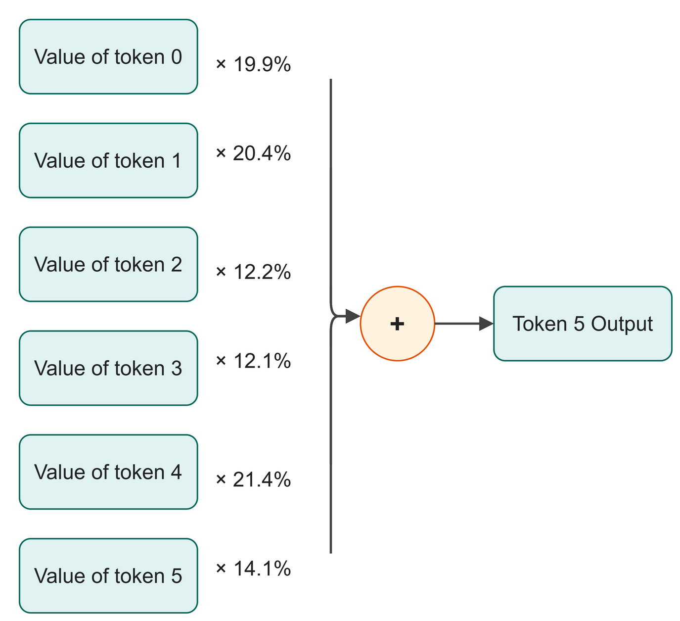Figure 6.2: Token 5 blends information from previous tokens.

Here is the "aha" moment: attention is nothing more than a weighted average (Figure 6.2). When token 5 calculates its final value, it does not just pick the single best token to look at. It mixes them all.

First, we multiply all Queries by all Keys (q @ k.transpose) to get an attention score for every pair. We scale these down by dividing by sqrt(head_size) (the size of each attention head, which is 32 here) so the numbers do not get too large. Then we apply softmax to turn these scores into percentages (weights) that sum to 1.0 (or 100%).

For example, when token 5 looks at the sequence, it might assign weights like this (as plotted in Figure 6.3). These values are rounded for display, so they add up to about 100% (100.1%):

Token 0: 19.9%
Token 1: 20.4%
Token 2: 12.2%
Token 3: 12.1%
Token 4: 21.4%
Token 5: 14.1%

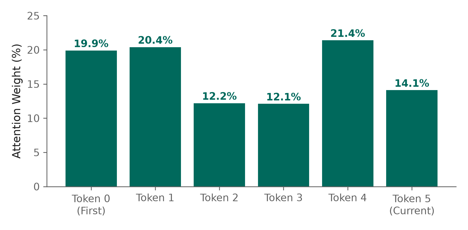Attention weights for token 5 Figure 6.3: A plotted bar chart of the attention weights.

Token 5's final output is simply 19.9% of the value of token 0, plus 20.4% of the value of token 1, and so on for all six tokens. The "Numbers Machine" builds context by blending the numbers of the most relevant past tokens. This context gathering completes the "Attention" stage of our map (Figure 6.1).

The Causal Mask¶

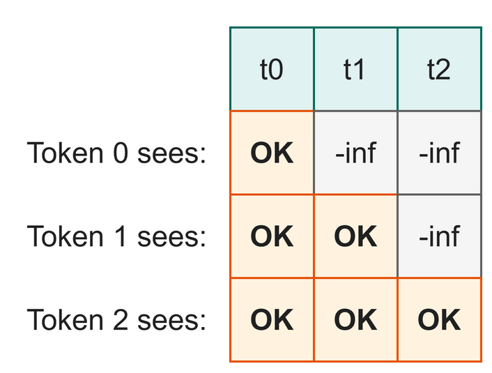The causal mask hides the future Figure 6.4: A lower triangular mask ensures tokens only see the past.

There is a catch: the model processes all tokens at once. If we let token 5 look at token 6, it would be cheating. During training, it would just copy the answer from the future instead of learning to predict it.

We apply a causal mask (a triangle of negative infinities, shown in Figure 6.4) to the scores before the softmax step. Softmax turns -infinity into exactly 0.0. This ensures that token 5 pays 0% attention to tokens 6, 7, 8, and 9. It can only see itself and the past.

In Business

When parsing a customer support chat, a simple keyword search treats every word independently. A context-aware system uses self-attention. It connects the word "refund" in message 4 back to the "broken screen" mentioned in message 1, understanding the full conversation history before it generates a reply in the company's house style.

Code¶

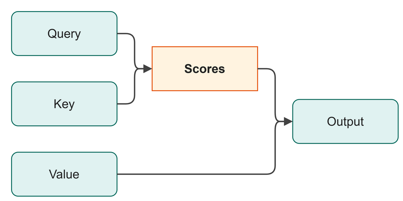How the code flows in self-attention Figure 6.5: The Q, K, V vectors are created, scored, masked, and then multiplied.

We use src/ch05_self_attention.py to build the SingleHeadAttention class (flow illustrated in Figure 6.5).

src/ch05_self_attention.py (excerpt)
        q = self.query(x)
        k = self.key(x)
        v = self.value(x)

        # Compute attention scores and scale them to keep variance stable
        scale = HEAD_SIZE ** -0.5
        scores = q @ k.transpose(-2, -1) * scale

        # Mask future tokens by setting their scores to negative infinity
        scores = scores.masked_fill(self.tril[:T, :T] == 0, float("-inf"))

        # Convert scores to probabilities and apply dropout
        weights = F.softmax(scores, dim=-1)
        weights = self.dropout(weights)

        # Compute final output by taking weighted sum of values
        out = weights @ v

Here is what happens when we run it:

Terminal

$ python src/ch05_self_attention.py
--- Attention weights (what token 5 attends to) ---
Token 5 attends to tokens 0..5 (future tokens masked):
  token 0: 0.199  #####
  token 1: 0.204  ######
  token 2: 0.122  ###
  token 3: 0.121  ###
  token 4: 0.214  ######
  token 5: 0.141  ####
  token 6: 0.000
  token 7: 0.000
  token 8: 0.000
  token 9: 0.000

Self-attention done! Ready for Chapter 7.

What just happened:

Lines 1 to 3 created independent Query, Key, and Value vectors.
Line 7 computed the attention scores between all tokens.
Line 10 masked the future tokens (notice tokens 6 to 9 have exactly 0.000 weight).
Line 17 created the output (for example, token 5 created its output by taking a weighted average of tokens 0 through 5).

Shape Check: Table 6.1 lists the shapes of the attention variables.

Table 6.1: Tensor shapes during the self-attention calculation.

Variable	Shape	Meaning
`q`, `k`, `v`	`[B, T, head_size]`	Queries, Keys, and Values. `head_size` is 32.
`scores`	`[B, T, T]`	Attention scores between every pair of tokens.
`weights`	`[B, T, T]`	The softmax probabilities (summing to 1 per row).
`out`	`[B, T, head_size]`	The final context-aware output vectors.

Try It¶

Try It

Remove the scale division in src/ch05_self_attention.py by changing it to scale = 1.0. Run it again. Notice how the weights become much more extreme (some very close to 1.0, others 0.0). The scaling is critical to keep the model flexible and learning smoothly.

Watch Out

Be careful with the transpose step. We only want to swap the last two dimensions (Time and head_size) to compute the dot product properly. If you use .T, it might flip the Batch dimension too, crashing your shape calculations. Always use .transpose(-2, -1).

Key Takeaways¶

Self-attention builds context by letting tokens "look" at other tokens.
The QKV system works like a search engine: Queries match with Keys to retrieve Values.
Attention is just a weighted average of the Values.
A causal mask sets future scores to negative infinity, preventing the model from cheating.

Check Your Understanding¶

What is the difference between a Query and a Key?
Why do we divide the attention scores by the square root of the head size?
What happens to a score of negative infinity when passed through softmax?
Why is the causal mask necessary for a language model?

Chapter 7: Multi-Head Attention¶

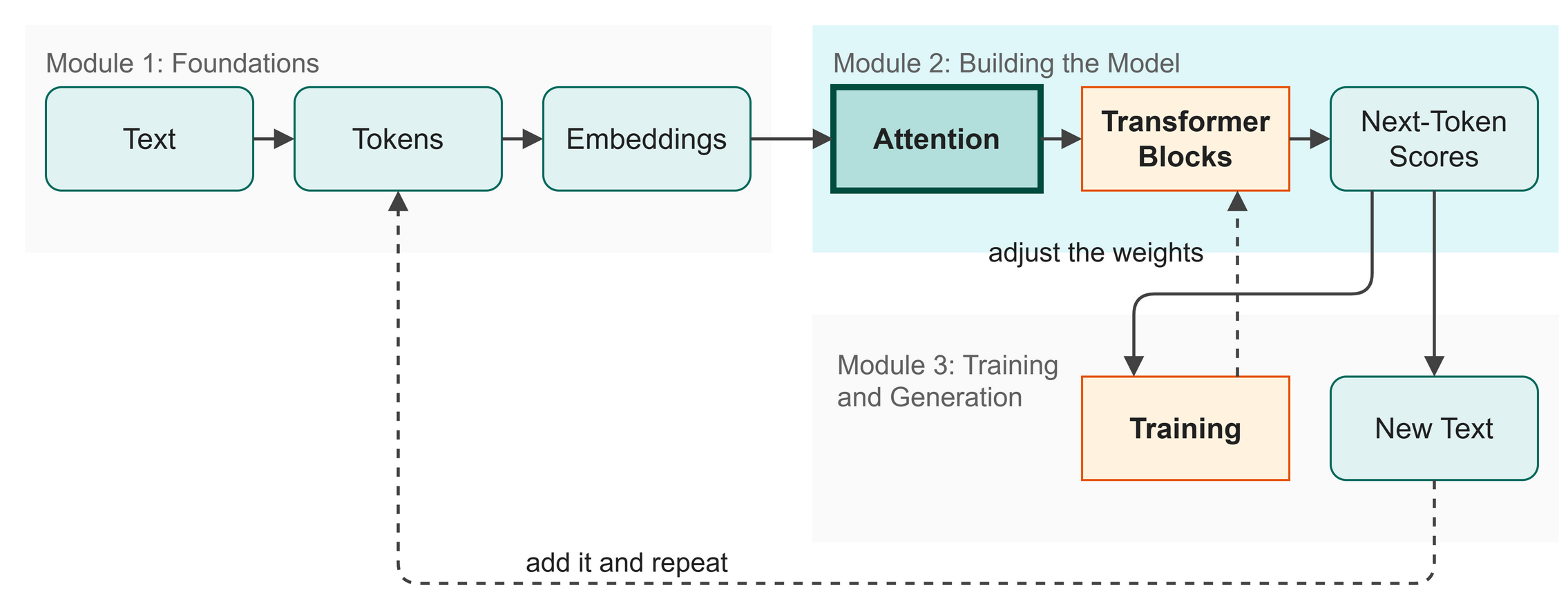Where we are in the big picture Figure 7.1: We run multiple attention heads at the same time to gather richer context.

In Chapter 6, we built one attention head. It acts as a single "reader" scanning the text. But one reader is rarely enough to catch everything. In this chapter you will:

Run multiple attention heads in parallel.
Understand how different heads learn to track different patterns.
Concatenate their outputs into a single rich representation.

Words to Know

Multi-Head Attention: Running several attention operations simultaneously.
Concatenation: Joining multiple vectors end-to-end to form a longer vector.
Projection: A linear layer that blends the concatenated outputs.

Theory¶

One Reader Isn't Enough¶

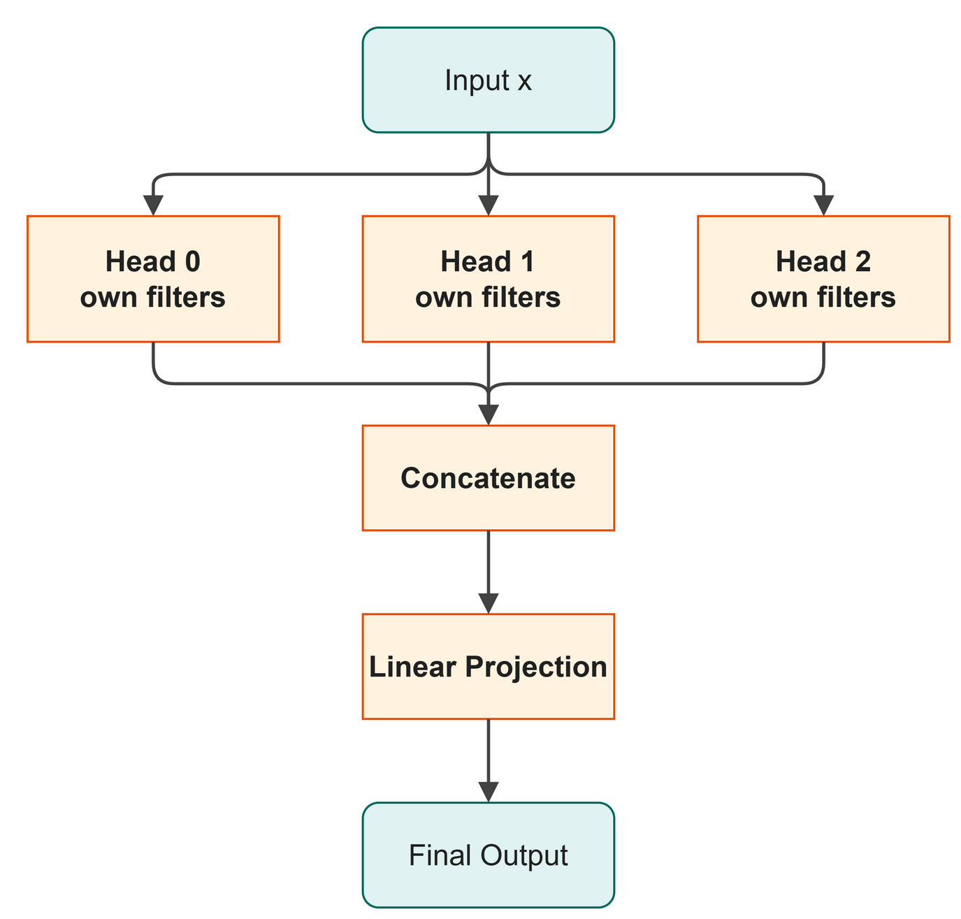Parallel heads looking at different features Figure 7.2: Every head sees the same input through its own filters, and their answers are joined rather than merged.

When you read a sentence, you track multiple things at once:

Who is the subject?
What action is happening?
What is the tone, serious or sarcastic?

A single attention head can only "look" for one kind of pattern at a time. Multi-head attention fixes this by running several heads in parallel, as shown in Figure 7.2. Think of it as a team of readers, each highlighting different details, who then combine all their notes.

How It Works¶

Multi-head attention simply repeats the mechanism from Chapter 6:

Run 4 independent SingleHeadAttention modules on the exact same input.
Each head produces an output of 32 numbers (head_size).
Glue (concatenate) all 4 outputs together: 4 heads × 32 numbers = 128 numbers.
Apply a final linear projection to blend them.

Because each head starts with different random weights (its own Q, K, and V filters), no two heads ever see the text the same way, and training pushes them further apart.

Why Four Heads and Not One Big One¶

Four readers sound expensive. They are not, and this is the part that surprises people.

A head's filters are sized by its head_size, not by the full 128 channels. Split 128 channels across four heads and each head gets filters that are a quarter as wide. Multiply it out and the totals match exactly:

src/examples/ch07_head_budget.py
head_size = C // n_heads

## Every head holds three filters (query, key, value), each C by head_size
four_heads = n_heads * 3 * C * head_size
one_head = 3 * C * C

Terminal

$ python src/examples/ch07_head_budget.py
4 heads of 32: 49,152 numbers
1 head of 128  : 49,152 numbers
Same budget: True

Four points of view cost the same as one. That is why every model in this family uses many heads: the split is free, so there is no reason to take one perspective when you can have four.

Do the Heads Really Differ?¶

That is the claim. Here is the check, on the model you will train in Chapter 13.

The script below loads the trained weights, feeds in a real line of Shakespeare, and prints how much attention the last character pays to each earlier character, one row per head.

src/examples/ch07_heads_differ.py (excerpt)
for h, head in enumerate(model.blocks[0].attn.heads):
    with torch.no_grad():
        scores = head.query(x) @ head.key(x).transpose(-2, -1) * head.head_size ** -0.5
        weights = F.softmax(scores, dim=-1)[0, -1]     # the last character's row

Terminal

$ python src/examples/ch07_heads_differ.py
Prompt: "JULIET: O Romeo"

Attention paid by the last character, one row per head:
              J    U    L    I    E    T    :    _    O    _    R    o    m    e    o
  head 0:  0.02 0.04 0.01 0.06 0.03 0.04 0.04 0.02 0.06 0.04 0.05 0.04 0.11 0.38 0.07
  head 1:  0.02 0.02 0.03 0.03 0.04 0.08 0.12 0.06 0.05 0.07 0.02 0.10 0.16 0.14 0.06
  head 2:  0.04 0.07 0.04 0.06 0.05 0.11 0.04 0.06 0.09 0.07 0.07 0.06 0.09 0.09 0.06
  head 3:  0.03 0.02 0.01 0.05 0.05 0.03 0.03 0.05 0.04 0.04 0.05 0.08 0.12 0.25 0.14

Sharpest focus per head: 0->'e' (0.38)  1->'m' (0.16)  2->'T' (0.11)  3->'e' (0.25)

Read the rows, not the labels. Head 0 commits: it puts 0.38 of its attention on the single character just before the end and largely ignores the rest. Head 3 does something similar but softer, splitting between e and the final o. Head 1 spreads itself over the colon, the m and the e, holding several places at once. Head 2 is nearly flat: its largest weight is 0.11 and its smallest is 0.04, which is close to paying equal attention to everything.

So the heads do differ, and not in the tidy way the textbook story suggests. One is sharp, one is soft, one is diffuse, and one is barely committing at all. That last one is worth sitting with: in a trained model, some heads do very little. Nobody assigned these roles, and nobody can promise that head 1 is the "grammar head". They are four different filters that started from four different random draws and were shaped by the same pressure to predict the next character.

Watch Out

It is tempting to read a story into each head: this one tracks subjects, that one tracks punctuation. Sometimes a head really is that clean, and researchers have found interpretable ones in large models. Often it is not, as head 2 shows. Look at the numbers before you tell the story.

The Output Projection¶

After concatenating the 4 heads, we pass the 128 numbers through one final linear layer (the proj layer).

Why? The heads might have found redundant or conflicting information. The projection layer learns to blend the insights: "if head 1 and head 3 agree on this pattern, emphasize it; if head 2 is unsure, ignore it." It mixes the 4 separate perspectives into a single unified context vector of 128 numbers. This completes the "Attention" stage of our map (Figure 7.1).

There is a simpler thing we could have done here, and it is worth seeing why we did not. We could average the four heads instead of gluing them end to end. Averaging would give us 32 numbers rather than 128, which sounds tidy, but it throws away exactly what we paid for. Head 0's sharp focus on one character and head 2's flat spread would cancel each other into a lukewarm middle. Concatenation keeps every head's answer intact and lets the projection layer decide what each one is worth. Averaging decides in advance that they are all worth the same.

In Business

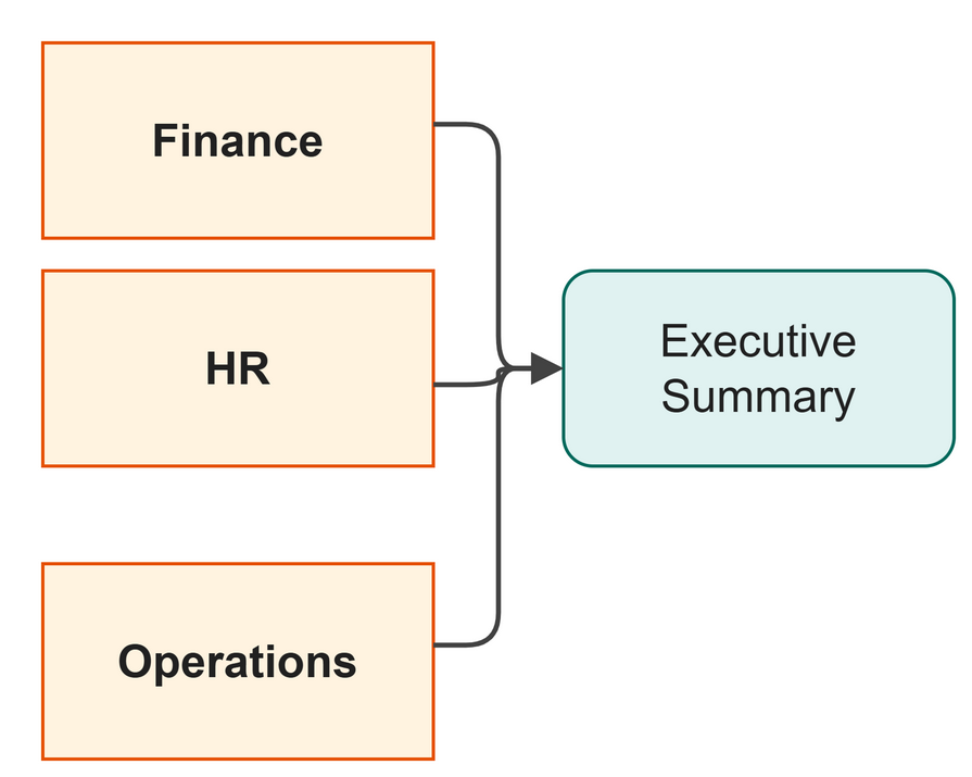Different departments form a single executive summary Figure 7.3: Multi-head attention gathers different perspectives.

When building an assistant to draft emails in your company's house style, you don't just look for one pattern. You track tone, structure, and vocabulary (Figure 7.3). Multi-head attention works exactly the same way: it asks 4 different "departments" to evaluate the text, then compiles a final executive summary.

Code¶

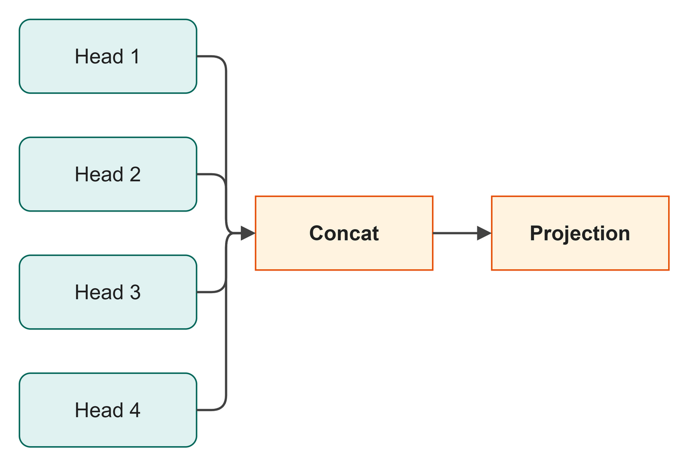How the code flows in multi-head attention Figure 7.4: The heads run in parallel, get concatenated, and projected.

We use src/ch06_multihead_attention.py to build the MultiHeadAttention class, as flow-charted in Figure 7.4.

src/ch06_multihead_attention.py (excerpt)
        # Run each head in parallel
        head_outputs = [h(x) for h in self.heads]

        # Concatenate outputs along the last dimension
        out = torch.cat(head_outputs, dim=-1)

        # Apply projection and dropout
        out = self.dropout(self.proj(out))

Here is what happens when we run it:

Terminal

$ python src/ch06_multihead_attention.py
--- Comparing one head vs multi-head ---
Single head output  shape: torch.Size([2, 10, 32])  (head_size=32)
Multi-head output   shape: torch.Size([2, 10, 128])  (C=128)

Multi-head output has 4x more channels - it sees 4 perspectives at once.

Multi-head attention done! Ready for Chapter 8.

What just happened:

Line 2 ran 4 independent attention heads at the same time.
Line 2's result is that each head produced an output with 32 channels.
Line 5 concatenated them, resulting in 128 channels (the original embedding dimension).
Line 8 applied projection and dropout so the final output matches the exact shape of the input.

Shape Check: Table 7.1 outlines the shape transformations through the heads.

Table 7.1: Tensor shapes during the multi-head attention step.

Variable	Shape	Meaning
`head_outputs`	4 × `[B, T, 32]`	A list of outputs from the 4 heads.
`out` (after cat)	`[B, T, 128]`	The 4 outputs joined end-to-end.
`out` (final)	`[B, T, 128]`	The blended representation, ready for the next step.

Try It¶

Try It

Change the number of heads in src/utils/config.py. Set n_heads = 8 instead of 4. Run the script again. Notice how the head_size automatically drops to 16, so the final concatenated size is still 128 (8 × 16 = 128). The model can have more perspectives, but each one has less detail.

Watch Out

For multi-head attention to work cleanly, your embedding dimension (n_embd) must be perfectly divisible by your number of heads (n_heads). If you try n_embd = 128 and n_heads = 5, the program will crash because it cannot divide the channels equally.

Key Takeaways¶

Multi-head attention runs several single-head attention modules in parallel.
Splitting the channels across heads costs nothing: four heads of 32 hold the same 49,152 numbers as one head of 128.
The heads do end up different, but not in a tidy way. In our trained model one head is sharp, one is soft and one is close to flat.
The outputs are concatenated, not averaged, so that no head's answer is diluted by the others before the projection can weigh it.
A final linear projection blends the separate perspectives.
The output shape [B, T, C] is exactly the same as the input shape, making it easy to stack layers.

Check Your Understanding¶

Why is one attention head not enough to understand complex text?
If n_embd = 256 and n_heads = 8, what is the head_size?
Four heads of 32 hold the same number of weights as one head of 128. Why does splitting cost nothing?
Why do we concatenate the heads rather than average them?
In the run above, head 2's attention was almost flat. What does that tell you about the claim that each head learns its own linguistic role?
What is the purpose of the final projection layer?

Chapter 8: Feed-Forward and Norms¶

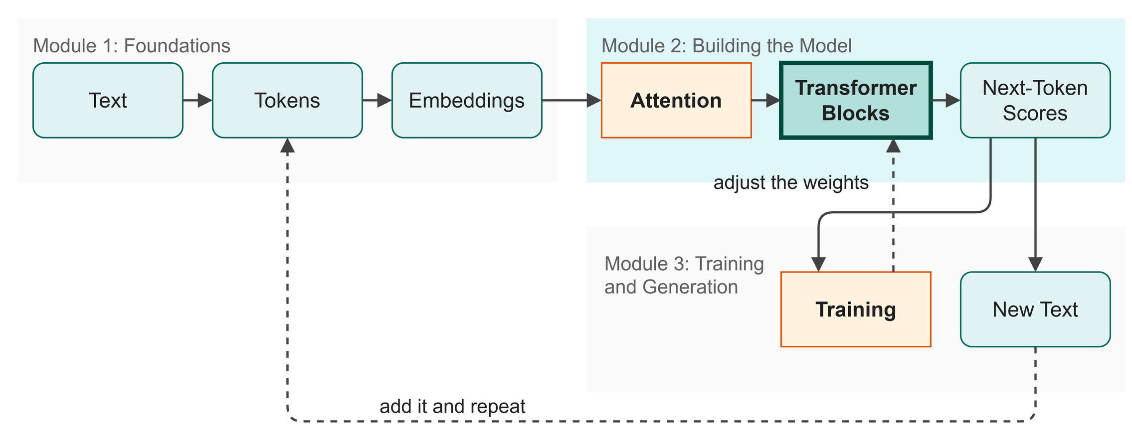Where we are in the pipeline Figure 8.1: We just built attention; now we process that context.

While attention (from Chapter 7) lets a token gather information from its neighbors, gathering information is only half the job. The token still needs to process that information and decide what to do with it. In this chapter you will:

Build a feed-forward network to process context.
Use a GELU curve to help the model learn smoothly.
Add Layer Normalization to keep the math stable.

Words to Know

Feed-Forward: A small neural network that processes each token independently.
GELU: A smooth curve that replaces negative numbers with near-zero values.
LayerNorm: A step that resets numbers to a safe size so training stays stable.

Theory¶

Thinking on Your Own¶

Attention is like listening to your team explain their ideas. Feed-forward is going back to your desk and thinking it over yourself.

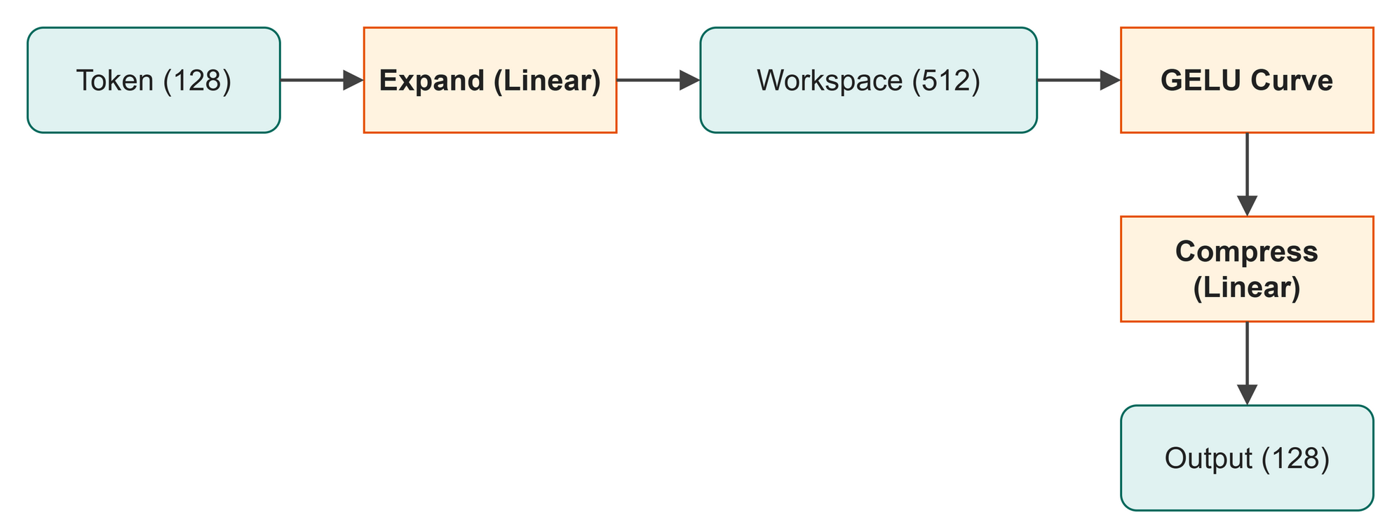A token goes through a wide workspace to process information Figure 8.2: The network expands to think, then compresses back to an answer.

The feed-forward layer is a small neural network applied to each token by itself (Figure 8.2). In our model, a token is a list of 128 numbers. The network first expands this to 512 numbers. This 4x expansion gives the model a wide workspace to spread out its calculations. After processing, it compresses the answer back down to 128 numbers.

The Smooth GELU Curve¶

Inside the feed-forward network, we apply a mathematical curve called GELU.

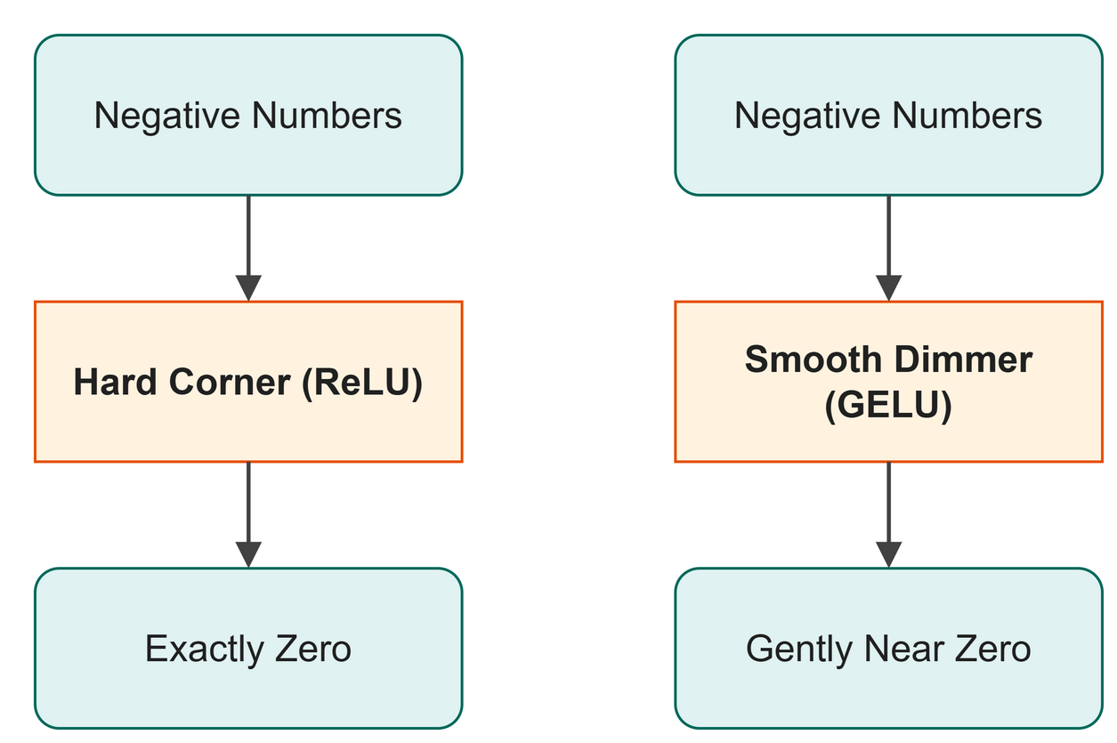ReLU creates a sharp corner while GELU makes a gentle curve Figure 8.3: GELU replaces a hard switch with a smooth dimmer.

A neural network needs a non-linear curve to learn complex patterns. An older choice is ReLU, which acts like a hard switch: negative numbers become exactly zero, while positive numbers stay the same.

GELU is a gradual dimmer switch, as seen in Figure 8.3. Strongly negative numbers become nearly zero. Numbers near zero are gently reduced. Positive numbers pass through almost unchanged.

During training, we use calculus to figure out how to adjust the model's weights. A hard corner like ReLU can produce sudden jumps that destabilize the math. GELU's smooth curve makes training much more stable. Most modern models use it.

Keeping Numbers Safe with LayerNorm¶

As numbers flow through many layers of a neural network, they can grow very large or shrink very small. Like compound interest, small multiplications add up quickly. Extremely large or small numbers break the training math.

Layer Normalization (LayerNorm) fixes this. It re-centers and re-scales the numbers for each token. After LayerNorm, the values average to 0 and have a standard spread of 1.

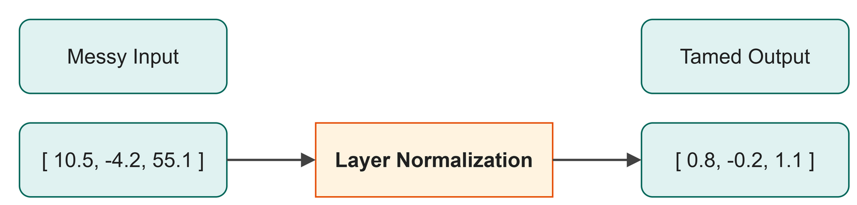A vector of varying numbers is scaled to have zero mean and standard variance Figure 8.4: LayerNorm centers messy numbers back around zero.

Think of it like resetting a runner's stopwatch after every lap (Figure 8.4). It does not change who is winning, but it keeps the numbers on the screen small and easy to read. In modern models, we apply LayerNorm before each major step. This gives the attention and feed-forward layers well-behaved numbers to work with.

Returning to the big picture map in Figure 8.1, the feed-forward network processes the context gathered by attention, and LayerNorm ensures the math remains stable before we pass the numbers to the next stage.

Code¶

src/ch07_feedforward.py (excerpt)
class FeedForward(nn.Module):
    def __init__(self):
        super().__init__()
        C = config.n_embd
        # A small neural network applied to each token independently
        self.net = nn.Sequential(
            nn.Linear(C, 4 * C),
            nn.GELU(),
            nn.Linear(4 * C, C),
            nn.Dropout(config.dropout),
        )

    def forward(self, x):
        return self.net(x)

Run the script to see the feed-forward layer and LayerNorm in action.

Terminal

$ python src/ch07_feedforward.py
--- GELU activation ---
GELU is like ReLU (zeros out negatives) but with a smooth curve.

  Input : [-3.0, -1.0, -0.5, 0.0, 0.5, 1.0, 2.0, 3.0]
  GELU  : [-0.004, -0.159, -0.154, 0.0, 0.346, 0.841, 1.954, 2.996]
  ReLU  : [0.0, 0.0, 0.0, 0.0, 0.5, 1.0, 2.0, 3.0]

--- Layer Normalization ---
LayerNorm re-centers and re-scales values at each position.

Before LayerNorm: mean=5.23, std=9.13
After  LayerNorm: mean=0.0000, std=1.0039

What just happened:

Lines 7 and 9 build a feed-forward network that expands from 128 to 512, then back to 128.
Line 8 applies GELU, which gently reduces negative numbers instead of snapping them to zero.
We passed messy numbers through LayerNorm and saw them neatly centered at zero with a standard spread of 1.

Shape Check:

Input to FeedForward: [Batch, Time, 128]
Output of FeedForward: [Batch, Time, 128]

Try It¶

Try It

Open src/ch07_feedforward.py and change the LayerNorm input to have a massive spread: x_single = torch.randn(config.n_embd) * 1000 + 500. Run the script again. You will see that LayerNorm still perfectly tames it back to a mean of 0 and a standard spread of 1.

In Business

Imagine you are building an assistant to draft company emails in your house style. If the system is unstable, it might output gibberish. LayerNorm acts like a manager double-checking work between steps, ensuring the data never drifts too far off track before passing it to the next team.

Key Takeaways¶

The feed-forward layer processes each token independently to build meaning.
It expands the token's data 4x to give itself room to think.
GELU provides a smooth mathematical curve to make training stable.
LayerNorm resets numbers to a safe size so deep networks do not break.

Check Your Understanding¶

Why does the feed-forward network expand its input size by 4?
What happens to a strongly negative number when it passes through GELU?
What is the average value of a token's numbers immediately after LayerNorm?

Chapter 9: The Transformer Block¶

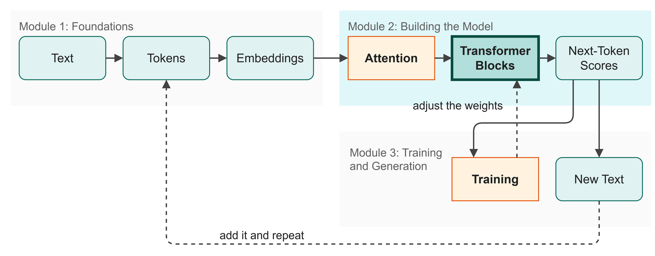Where we are in the pipeline Figure 9.1: We combine our pieces into a reusable building block.

After processing information with feed-forward and normalizing the math in Chapter 8, we now have all the ingredients: multi-head attention (where tokens talk to each other), feed-forward layers (where tokens think for themselves), and LayerNorm (to keep training stable). In this chapter you will:

Combine these parts into a single Lego brick called a Transformer block.
Add residual connections so deep networks can learn effectively.
Stack multiple blocks to build depth.

Words to Know

Transformer Block: A reusable block of code containing attention, feed-forward, and normalization.
Residual Connection: A shortcut that lets information skip a step, keeping the original signal intact.

Theory¶

Putting the Pieces Together¶

A single Transformer block combines our tools into a powerful unit. The forward pass of one block is just two simple lines of code:

x = x + self.attn(self.ln1(x))  # "listen, then add to what I know"
x = x + self.ff(self.ln2(x))    # "think, then update what I know"

Notice the x = x + ... pattern. This is the secret to making deep neural networks work.

Trick 1: The Residual Connection¶

Instead of completely replacing a token's data with the output of the attention layer, we add the new information to the original data. This is called a residual connection (or skip connection), as seen in Figure 9.2.

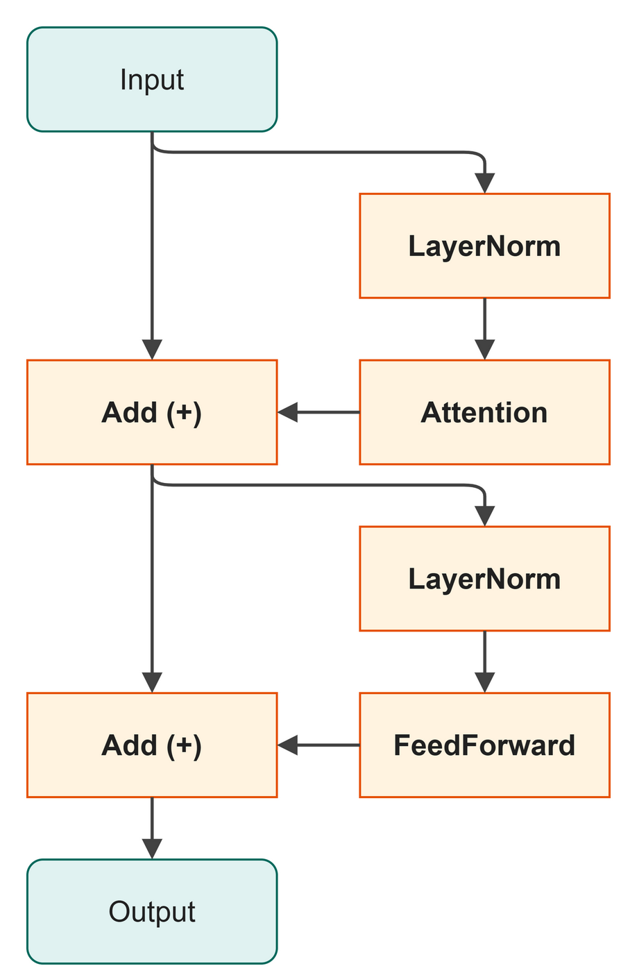The data flows down a main highway, taking side trips for attention and feed-forward Figure 9.2: Residual connections provide a direct highway through the block.

Why does this matter? Imagine you are in a game of telephone. Each person translates the message and passes it on. After 10 rounds, the original message is usually unrecognizable. Residual connections are like passing the original written message alongside the game of telephone. Even if the spoken message gets mangled, the original is still there.

During training, feedback signals travel backward through the layers to adjust weights. Without residual connections, this feedback must pass through every layer in sequence. If each layer distorts the signal slightly, the signal either grows too large or shrinks to nearly nothing. The direct +x highway allows feedback to travel cleanly through dozens of stacked layers.

Trick 2: Pre-Layer Norm¶

Notice that we apply LayerNorm before each major step: attention(LayerNorm(x)).

This is the modern "pre-norm" convention used in GPT models (Figure 9.3). We normalize the data first, then do the hard work. It ensures that attention and feed-forward always receive well-behaved numbers, stabilizing training in the early stages.

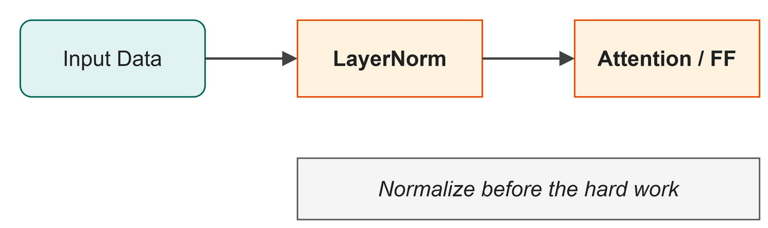Data passes through LayerNorm before entering the Attention layer Figure 9.3: Normalize the data before the hard work.

Stacking Blocks¶

One Transformer block is powerful, but not enough. We stack multiple blocks in sequence (Figure 9.4). Our model uses 4 blocks.

Each block refines the token representations further. Think of it like reading a complex document multiple times. First pass: "who are the characters?" Second pass: "what are their motivations?" Third pass: "what are the themes?" Earlier blocks capture simple patterns, while later blocks capture deeper meaning. This is why deeper models perform better.

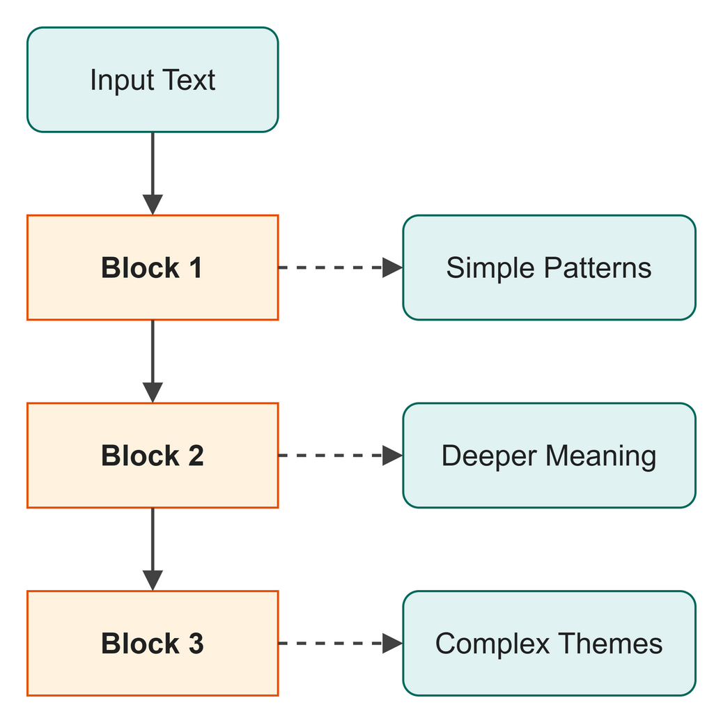Multiple blocks stacked on top of each other, building deeper understanding Figure 9.4: Stacking blocks allows the model to find complex patterns.

Returning to the big picture map in Figure 9.1, these stacked Transformer blocks form the core engine of our model, ready to process the embeddings into deep, contextualized representations.

Code¶

src/ch08_transformer_block.py (excerpt)
class TransformerBlock(nn.Module):
    def __init__(self):
        super().__init__()
        self.attn = MultiHeadAttention()
        self.ff   = FeedForward()
        # Layer normalization applied before attention and feed-forward
        self.ln1  = nn.LayerNorm(config.n_embd)
        self.ln2  = nn.LayerNorm(config.n_embd)

    def forward(self, x):
        # The + creates a residual connection, adding new info
        x = x + self.attn(self.ln1(x))
        x = x + self.ff(self.ln2(x))
        return x

Run the script to see a block process data and to check the parameter count.

Terminal

$ python src/ch08_transformer_block.py
One TransformerBlock parameters: 197,888
  MultiHeadAttention : 65,664
  FeedForward        : 131,712
  LayerNorms (x2)    : 512

Input  shape: torch.Size([2, 10, 128])
Output shape: torch.Size([2, 10, 128])   (same as input)

--- Residual connection demonstration ---
The input is never lost -- it always flows through.

Original token norm  : 11.470
Attention output norm: 4.599
After residual norm  : 12.903  (combined)

--- Stacking multiple blocks ---
Stacking 4 blocks:
  Params per block: 197,888
  Total params    : 791,552  (4 x 197,888)

Input  shape: torch.Size([2, 10, 128])
Output shape: torch.Size([2, 10, 128])  (unchanged after 4 blocks)

What just happened:

Lines 4 through 8 build a block containing attention, feed-forward, and LayerNorm.
Line 12 shows the residual connection combine the original token data with the attention output.
We stacked 4 blocks and saw the data flow through smoothly.

Shape Check:

Input to TransformerBlock: [Batch, Time, 128]
Output of TransformerBlock: [Batch, Time, 128]

The block is shape-preserving. The input and output have identical shapes, which is exactly what allows us to stack them endlessly like Lego bricks.

Try It¶

Try It

Open src/ch08_transformer_block.py and change the number of layers in the stack from config.n_layers to 12. Run the script again. Notice how the total parameter count grows, but the output shape remains exactly the same.

In Business

When building software systems (like a house-style writing assistant), you want modular, scalable processes. A Transformer block is the ultimate modular unit. If your assistant is not smart enough, you do not have to invent a new architecture; you just stack more blocks and train it longer.

Key Takeaways¶

A Transformer block combines LayerNorm, attention, and feed-forward layers.
Residual connections (x + ...) create a direct highway for data, allowing deep models to learn effectively.
Pre-norm applies LayerNorm before the hard work, stabilizing the math.
Blocks preserve the shape of the data, allowing us to stack them modularly.

Check Your Understanding¶

Why do we add the attention output to the original input (x + attention)?
What does "pre-norm" mean?
Why does the Transformer block output exactly the same shape it took in?

Chapter 10: The Full GPT Architecture¶

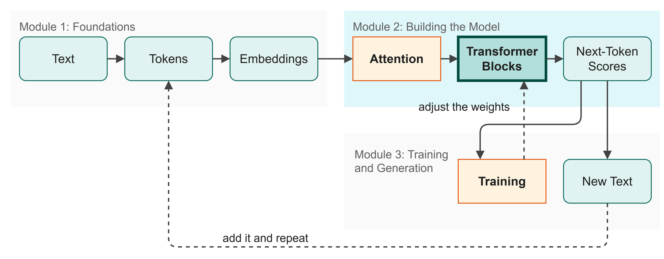Where we are in the pipeline Figure 10.1: We connect everything to output a prediction.

Now that we have built all the core components of a Transformer model in previous chapters, we can assemble them (Figure 10.1). In this chapter you will:

Build the full GPT model from end to end.
See how data flows through the entire pipeline.
Understand the final raw scores, called logits.

Words to Know

LM Head: The final linear layer that maps internal numbers back to vocabulary words.
Logits: The raw scores the model outputs for each possible next token.

Theory¶

The Final Assembly¶

The complete GPT model is surprisingly simple once you have the pieces.

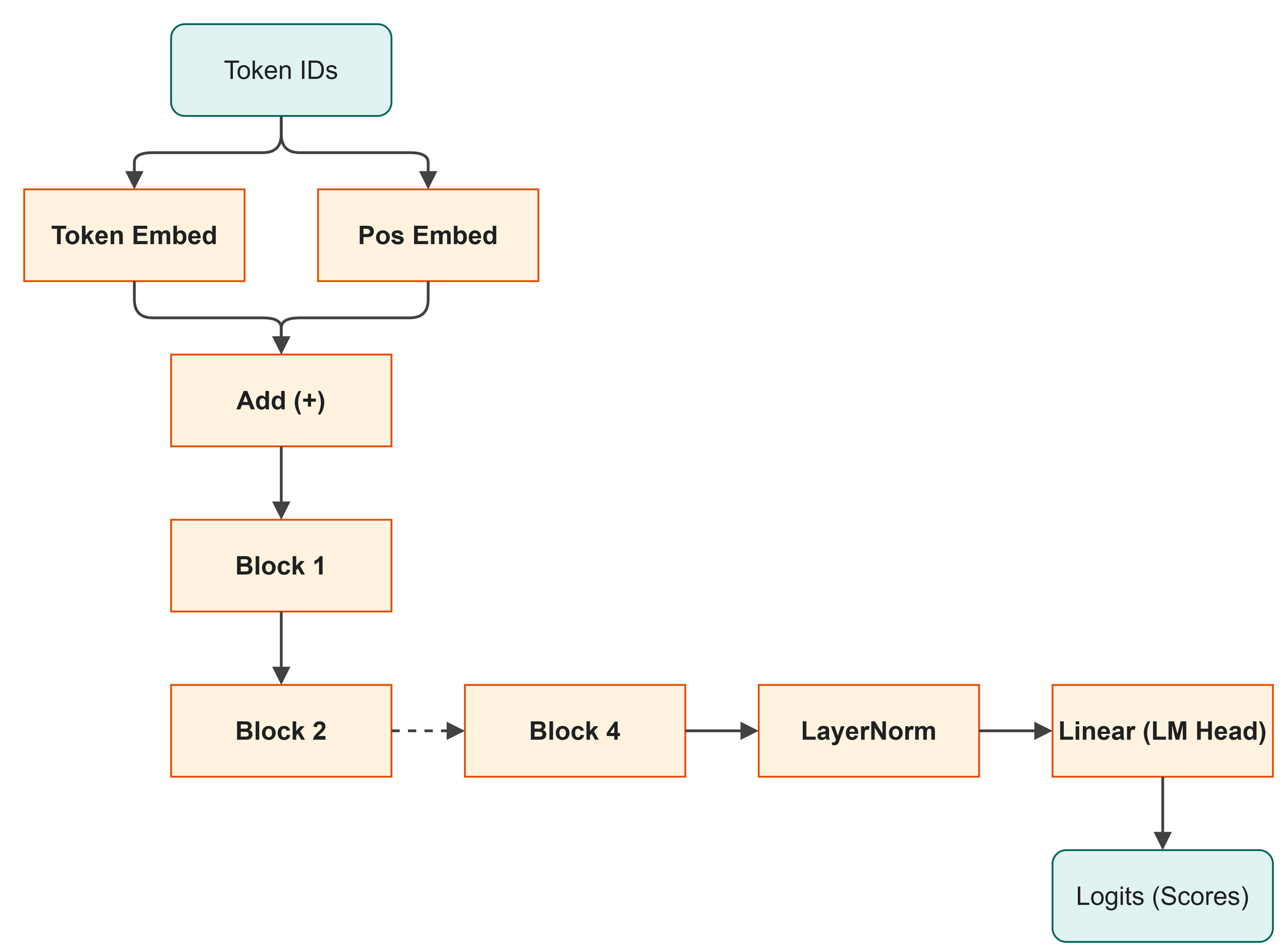The pipeline flows from embeddings through blocks to the LM head Figure 10.2: The full forward pass of the GPT model.

It flows exactly like a production assembly line (as shown in Figure 10.2):

Turn text into a list of numbers (Token IDs).
Look up the meaning and position vectors (Embeddings).
Process them through a stack of Transformer blocks.
Tidy up the numbers one last time (Final LayerNorm).
Map the internal 128 numbers back to the 65 possible characters (LM Head).

Tracing the Flow¶

Let's trace a concrete example. Suppose we feed the model the word "ROMEO" (5 tokens).

Step 1: Input The input is [30, 27, 25, 17, 27]. These are the specific token IDs for the characters "ROMEO", where 'R' is 30, 'O' is 27, 'M' is 25, and 'E' is 17 according to our vocabulary.

Step 2: Embeddings The model converts these 5 IDs into 5 rich vectors (128 numbers each), combining both meaning and position.

Step 3: Transformer Blocks The data passes through 4 blocks. After 4 blocks, the token O (at the end) has looked at all the previous letters. Its 128 numbers now encode something like "I am the last letter of a name from a famous play."

Step 4 & 5: Final Output A final LayerNorm stabilizes the numbers. Then, the LM Head (Language Model Head) takes those 128 numbers and projects them to 65 numbers. Why 65? Because our Shakespeare dataset has exactly 65 unique characters.

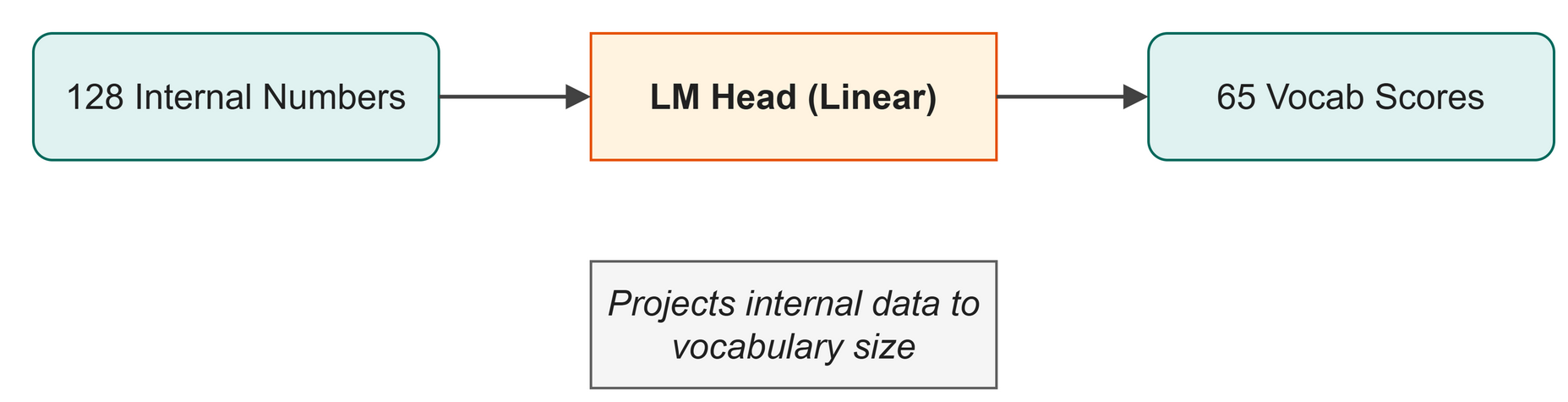The internal 128 numbers are projected to 65 vocabulary scores Figure 10.3: The LM Head projects internal data back to our vocabulary.

As Figure 10.3 illustrates, the model outputs 65 scores for every single token in the sequence. Each position independently predicts the character that comes next. The highest score at the final position is the model's best guess for what comes after "ROMEO".

What Are Logits?¶

The 65 scores the LM Head outputs are called logits.

Logit is a technical term for "raw score" (Figure 10.4). These numbers can be negative, zero, or very large. They do not add up to 1, so they are not probabilities yet. In Chapter 11, we will convert these raw scores into proper percentages to generate text. For now, just know that a higher logit means the model is more confident in that character.

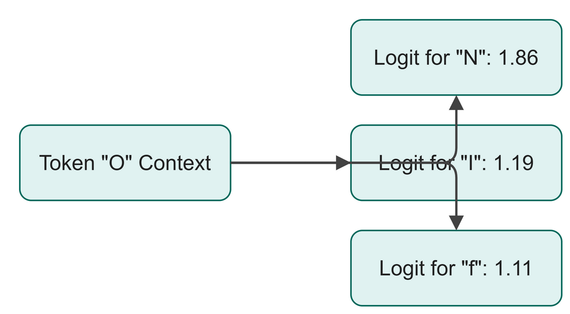Logit scores for the token O show highest confidence for N and I Figure 10.4: Logits are the raw scores for the next character.

Returning to the big picture map in Figure 10.1, we have built everything from Text to Next-Token Scores. The model is fully assembled, but right now it only outputs random guesses. We need to train it.

Code¶

src/ch09_gpt_model.py (excerpt)
class GPT(nn.Module):
    def __init__(self, cfg: GPTConfig):
        super().__init__()
        self.cfg = cfg

        # Look up table for token vectors
        self.token_emb = nn.Embedding(cfg.vocab_size, cfg.n_embd)
        # Look up table for position vectors
        self.pos_emb = nn.Embedding(cfg.block_size, cfg.n_embd)

        # A sequence of transformer blocks
        self.blocks = nn.Sequential(*[
            TransformerBlock() for _ in range(cfg.n_layers)
        ])

        # Final layer normalization and linear layer to output scores
        self.ln_f = nn.LayerNorm(cfg.n_embd)
        self.lm_head = nn.Linear(cfg.n_embd, cfg.vocab_size, bias=False)

    def forward(self, token_ids):
        B, T = token_ids.shape
        assert T <= self.cfg.block_size, \
            f"Sequence length {T} exceeds block_size " \
            f"{self.cfg.block_size}"

        tok_emb = self.token_emb(token_ids)
        positions = torch.arange(T, device=token_ids.device)
        pos_emb = self.pos_emb(positions)

        # Combine token and position embeddings
        x = tok_emb + pos_emb

        # Pass through the transformer blocks
        x = self.blocks(x)

        # Final normalization and produce scores
        x = self.ln_f(x)
        logits = self.lm_head(x)
        return logits

Run the script to see the parameter breakdown and a test run.

Terminal

$ python src/ch09_gpt_model.py
Model parameter breakdown:
  Token embedding  :      8,320
  Position embedding:    16,384
  4 Transformer blocks:   791,552
  LM head          :      8,320
  LayerNorm (final):        256
  ---
  TOTAL            :    824,832

Input  shape: torch.Size([2, 10])   (B, T)
Output shape: torch.Size([2, 10, 65])  (B, T, vocab_size)

At each position, model outputs 65 scores.
The highest score = best guess for next character.

First position logits (top 5 scores):
  token 26: 1.861
  token 21: 1.195
  token 44: 1.118
  token 57: 1.071
  token 34: 0.972

Note: these are random (untrained model).

What just happened:

Line 1 assembles the complete GPT class.
Line 12 creates the blocks that give us exactly 824,832 parameters (weights). The original GPT-2 Small had 117 million. Our model uses the exact same architecture, just scaled down.
Line 38 finishes the forward pass, where the model outputs 65 logits (scores) for each position.

Shape Check:

Input token IDs: [Batch, Time]
Output logits: [Batch, Time, 65] (Vocab size is 65)

Try It¶

Try It

Open src/ch09_gpt_model.py and modify config.n_layers = 6 just to test. Run the script again. Watch how the parameter count increases. The blocks contain the vast majority of the model's "brain".

In Business

Building the final GPT architecture is like assembling a complete production pipeline from modular components. In our house-style writing assistant, we combine a data reader (embeddings), an analysis engine (the blocks), and an output formatter (the LM head). Because it is modular, you can upgrade the engine (add more layers) without rewriting the rest of the pipeline.

Key Takeaways¶

The full model stacks embeddings, Transformer blocks, and a final LM head.
The LM head is a linear layer that projects the internal representations back to the vocabulary.
The model outputs logits, which are raw, un-normalized scores for the next token.
Our complete model has ~825K parameters, proving that powerful architectures can be built at a small scale.

Check Your Understanding¶

If the input sequence has 10 tokens, how many predictions does the model make?
Why does the LM head output exactly 65 numbers per token?
What is a logit?

Chapter 11: Causal Language Modeling¶

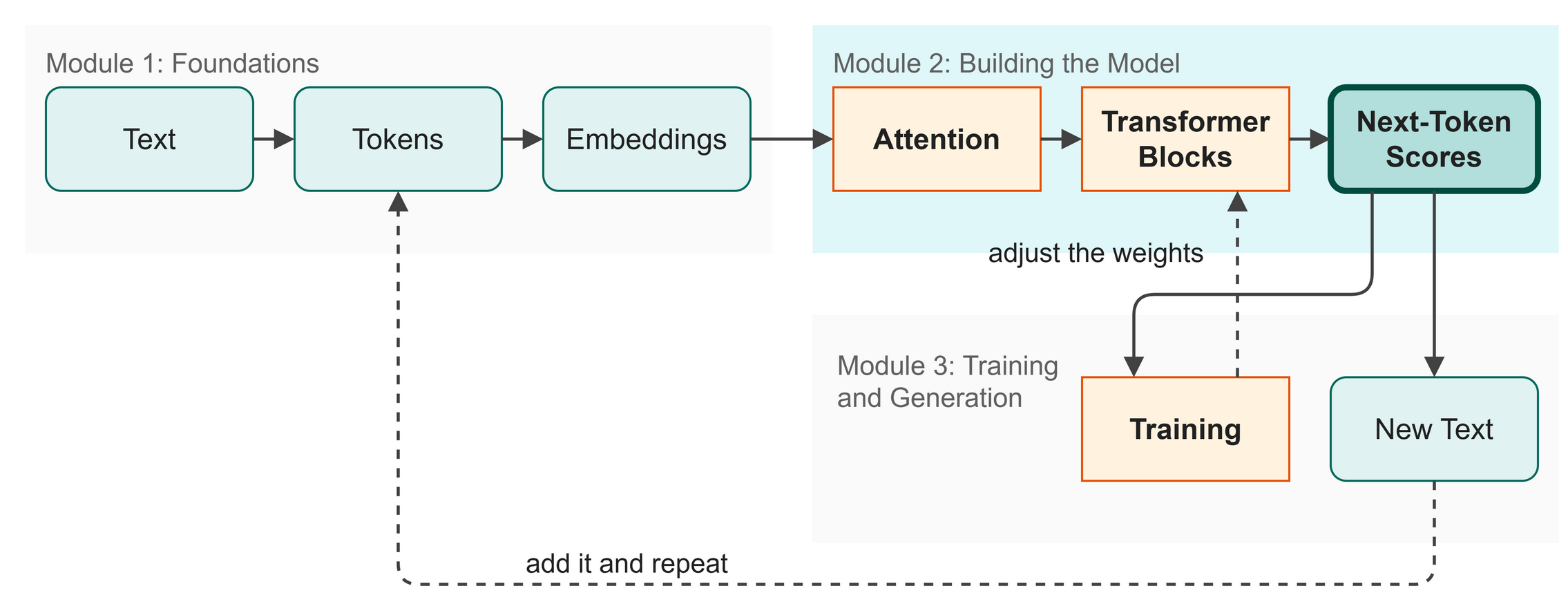You are here: Next-Token Scores Figure 11.1: The model is built. Now we define its goal: predicting the next token.

Now that we have assembled the full Transformer architecture in Chapter 10, our engine is built. But an engine is useless without a task (Figure 11.1). In this chapter, we give our model its objective: causal language modeling. This simply means guessing the next token based only on what came before it. We will also learn how to measure its performance.

In this chapter you will:

Shift the training sequence to create input and target pairs.
Understand cross-entropy loss as a measure of surprise.
See how generation is just a loop of predicting and appending.

Words to Know

Logits: The raw, unnormalized scores the model outputs before they are turned into probabilities.
Softmax: A mathematical function that squashes a list of any numbers into positive percentages that add up to 100%.
Cross-Entropy Loss: A mathematical way to measure how wrong the model's predictions are. Lower is better.
Autoregressive: A process that uses its own past outputs as inputs for its next step.

Theory¶

The Training Trick: One Pass, Many Examples¶

How do we train a model to predict the next token? You might think we feed it one token, ask for the next, check the answer, and then feed it two tokens. That would be incredibly slow.

The brilliant insight of causal language modeling is that a single pass over a sequence of length T gives us T training examples all at once.

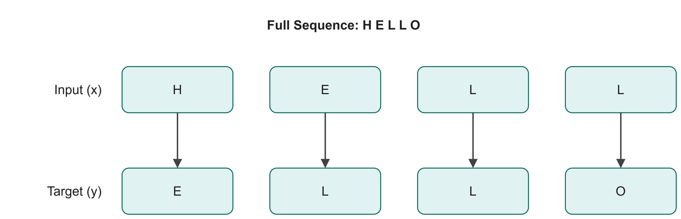Sequence shifted to create targets Figure 11.2: One sequence provides multiple training examples simultaneously.

As shown in Figure 11.2, the model processes the whole sequence. Because of the causal mask (from Chapter 6), position 2 cannot see position 3. Each position only sees what came before it. Therefore, at every single position, the model can make a valid prediction about what comes next.

Input and Target: The Shifted Pair¶

To implement this efficiently, we take our sequence of text and create two slightly different copies:

Input (x): The sequence missing its very last token.
Target (y): The sequence missing its very first token.

This means that at any position i, the character in the input $x[i]$ is supposed to predict the character in the target $y[i]$. If our sequence is "HELLO", x is "HELL" and y is "ELLO". At position 0, "H" predicts "E". At position 1, "E" (with "H" as context) predicts "L", and so on.

Logits and Probabilities¶

When our model makes predictions, it does not immediately output a single character or a clean percentage. It outputs raw numbers called logits.

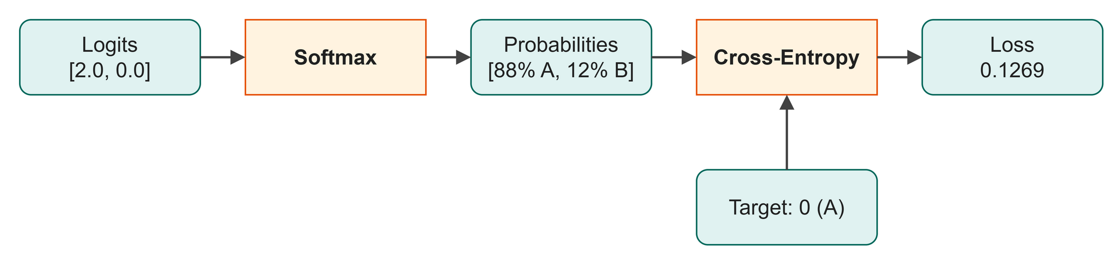Logits turned into probabilities and loss Figure 11.3: Softmax converts raw scores into valid percentages.

Logits can be any number: negative, positive, small, or large. To make sense of them, as illustrated in Figure 11.3, we pass them through a function called softmax. Softmax squashes all the logits so they are positive and sum to exactly 1.0 (or 100%). Now we have a probability distribution over our 65 possible characters.

Measuring Success: Cross-Entropy Loss¶

Once we have probabilities, we need to know how well the model is doing. We use a metric called cross-entropy loss.

Think of loss as a measure of the model's surprise. If the correct next character is "A", and the model assigned a 99% probability to "A", it is not surprised at all. The loss is very low. If it assigned a 1% probability to "A", it is highly surprised. The loss is very high.

If a model is completely untrained and guessing blindly among our 65 characters, it will assign roughly equal probability (about 1.5%) to each. The mathematical loss for this complete ignorance is about 4.17. We want our training process to push this number down.

This brings us to the end of the "Next-Token Scores" stage on our map. Our model now makes predictions and measures its own mistakes, setting the stage for it to learn.

Code¶

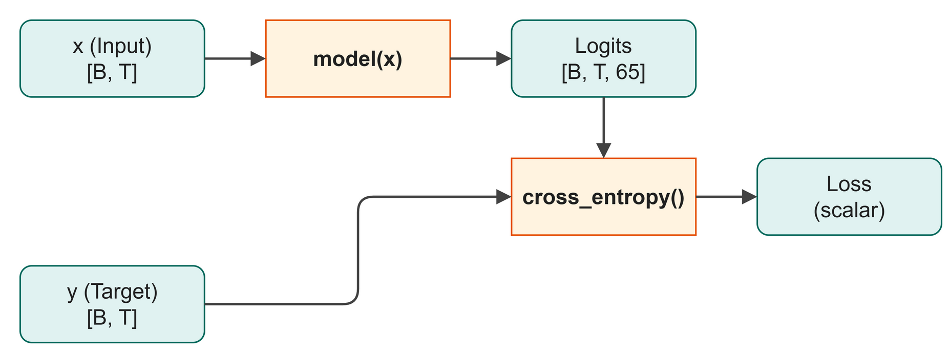Code flow: logits and targets into cross-entropy Figure 11.4: The model produces logits for the input, which are compared to the target to calculate loss.

Let's look at how this is implemented (following the flow in Figure 11.4).

src/ch10_causal_lm.py (excerpt)
    x = example_ids[:-1]
    y = example_ids[1:]

    logits = model(token_ids)

    # Calculate loss by comparing predictions to actual targets
    loss = F.cross_entropy(
        logits.view(B * T_len, config.vocab_size),
        targets.view(B * T_len)
    )

And how to run the full script:

Terminal

$ python src/ch10_causal_lm.py
--- 1. Constructing input/target pairs ---
Sequence: [20, 17, 30, 30, 33, 1, 35, 53, 56, 30]
Input  x: [20, 17, 30, 30, 33, 1, 35, 53, 56]
Target y: [17, 30, 30, 33, 1, 35, 53, 56, 30]
At each position i, x[i] predicts y[i].

--- 2. Computing cross-entropy loss ---
Logits shape : torch.Size([4, 20, 65])
Targets shape: torch.Size([4, 20])
Loss (random model): 4.3070
Expected loss for random: 4.1744

--- 3. Text generation ---
We extend a starting sequence one token at a time.

Generated IDs (first 10): [0, 54, 34, 5, 55, 18, 63, 52, 43, 10]
Output shape: torch.Size([1, 51])
After training (Chapter 13), this will produce real text!

What just happened:

Lines 1 and 2 slice a short sequence of 10 tokens into an input x of length 9 and a target y of length 9 to demonstrate input/target pairs.
Line 4 passes a random batch of 20 tokens into the untrained model to get logits for the loss computation step.
Lines 7 to 10 calculate the cross-entropy loss, which is 4.3070, very close to our expected random guessing loss of 4.1744.
The output shows we generated 50 tokens. The machinery works; the weights are still random, so the characters are too.

Shape Check:

(Note: The shapes below are from the loss computation step, which uses 20 tokens, unlike the 10-token sequence used earlier. Table 11.1 lists the shapes at each step.)

Table 11.1: Tensor shapes for the cross-entropy loss calculation.

Variable	Shape	Meaning
`token_ids`	`[4, 20]`	4 batches of 20 tokens each.
`logits`	`[4, 20, 65]`	A score for each of the 65 possible next characters, at every position.
`loss`	`[]`	A single scalar number representing the average surprise.

Try It¶

How does confidence affect the loss? We can simulate different prediction scenarios manually.

src/examples/ch11_loss_demo.py
"""Calculate cross-entropy loss for different confidence levels."""
import torch
import torch.nn.functional as F

## Two possible words: 'A' (index 0) or 'B' (index 1)
target = torch.tensor([0]) # The correct answer is 'A'

print("Scenario 1: Guessing blindly (50% / 50%)")
logits_blind = torch.tensor([[0.0, 0.0]])
loss_blind = F.cross_entropy(logits_blind, target)
print(f"Loss: {loss_blind.item():.4f}")

print("\nScenario 2: Confident and right (88% for 'A')")
logits_right = torch.tensor([[2.0, 0.0]])
loss_right = F.cross_entropy(logits_right, target)
print(f"Loss: {loss_right.item():.4f}")

print("\nScenario 3: Confident and wrong (88% for 'B')")
logits_wrong = torch.tensor([[0.0, 2.0]])
loss_wrong = F.cross_entropy(logits_wrong, target)
print(f"Loss: {loss_wrong.item():.4f}")

Lines 14 and 15 calculate the loss when the model is confident and correct, resulting in a much lower loss.

Terminal

$ python src/examples/ch11_loss_demo.py
Scenario 1: Guessing blindly (50% / 50%)
Loss: 0.6931

Scenario 2: Confident and right (88% for 'A')
Loss: 0.1269

Scenario 3: Confident and wrong (88% for 'B')
Loss: 2.1269

Try It

Open src/examples/ch11_loss_demo.py. Change logits_right to [[5.0, 0.0]] to make the model even more confident. Run the script and see how close to zero the loss gets.

In Business

Imagine you are building an assistant to draft text in your company's house style. Causal language modeling is how the assistant learns to write like you. By reviewing thousands of past emails and reports (the target sequences), it learns which words typically follow other words in your organization's specific context. The loss tells you how close its drafts are to your actual historical data.

Watch Out

When calculating cross-entropy loss in PyTorch, the F.cross_entropy function expects the logits to be flattened. It wants a 2D tensor of shape [Total Tokens, Vocabulary Size], not a 3D tensor of [Batch, Time, Vocabulary Size]. That is why the code uses logits.view(B * T_len, config.vocab_size). Forgetting to reshape is a very common bug!

Key Takeaways¶

A single forward pass on a sequence of length T provides T separate training examples, making training highly efficient.
The target sequence is simply the input sequence shifted one position into the future.
The model outputs raw logits, which softmax converts into probabilities.
Cross-entropy loss measures how "surprised" the model is by the correct answer. We want this number to be as low as possible.
An untrained model guessing among 65 characters will have a loss of approximately 4.17.

Check Your Understanding¶

If your sequence is "DATA", what is the input sequence x and the target sequence y?
Why do we need softmax before we can interpret the model's output as percentages?
If a model is perfectly confident and perfectly correct, what should its cross-entropy loss be?

Module 3: Training and Generation¶

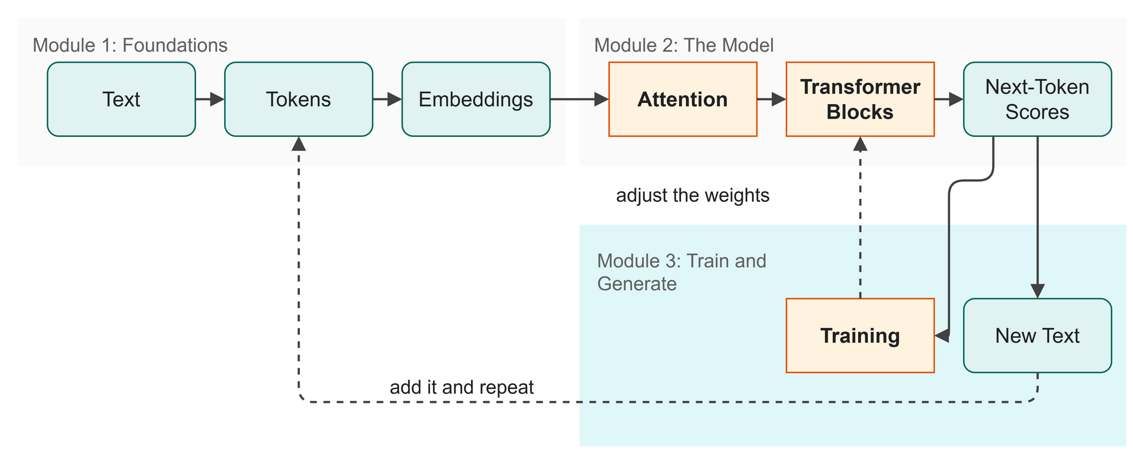Module 3 Map Figure M3.1: Training and Generation in the big picture.

With the engine built, it is time to turn it on. For a business use case, this is where we train the house-style assistant on your company's specific archive and then deploy it to generate value. We will feed it Shakespeare, teach it to write, and explore how to control its creativity.

In this module you will:

Prepare a dataset and data loader for training
Write the training loop that improves the model
Save your progress using checkpoints
Learn how greedy and sampling generation work
Use temperature and top-k to control text creativity
Put it all together into a complete pipeline

Chapters¶

Chapter 12: Dataset and DataLoader
Chapter 13: The Training Loop
Chapter 14: Checkpointing
Chapter 15: Greedy and Sampling
Chapter 16: Temperature and Top-k
Chapter 17: Putting It All Together

Chapter 12: Dataset and DataLoader¶

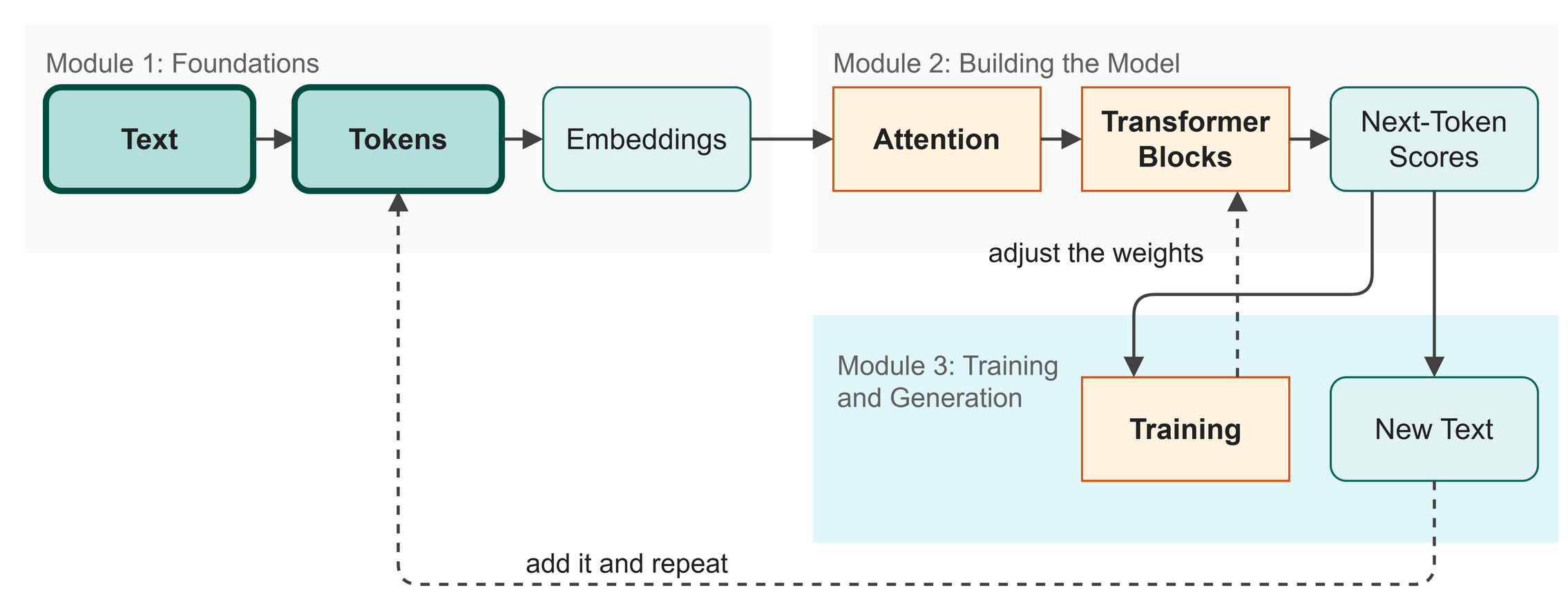You are here: Training Figure 12.1: We begin the training module by preparing our data pipeline.

We have our model, and we know our goal is to predict the next token (from Chapter 11). Now we need to feed data into the engine. Instead of pushing one character at a time, we will feed the model thousands of examples simultaneously. In this chapter, we build a pipeline to prepare and batch our Shakespeare dataset.

In this chapter you will:

Use a sliding window to generate training examples.
Understand how batches process multiple sequences in parallel.
Build a PyTorch Dataset and DataLoader.

Words to Know

Block Size: The maximum number of tokens the model can look at at one time (its context window).
Batching: Grouping multiple training examples together and processing them at the same time.
Dataset: A PyTorch class that defines how to retrieve a single training example.
DataLoader: A PyTorch utility that automatically groups individual examples into batches and shuffles them.

Theory¶

The Sliding Window¶

In the last chapter, we saw how a single sequence provides multiple training examples. But how do we extract these sequences from a massive text file like the complete works of Shakespeare?

We use a sliding window (Figure 12.2).

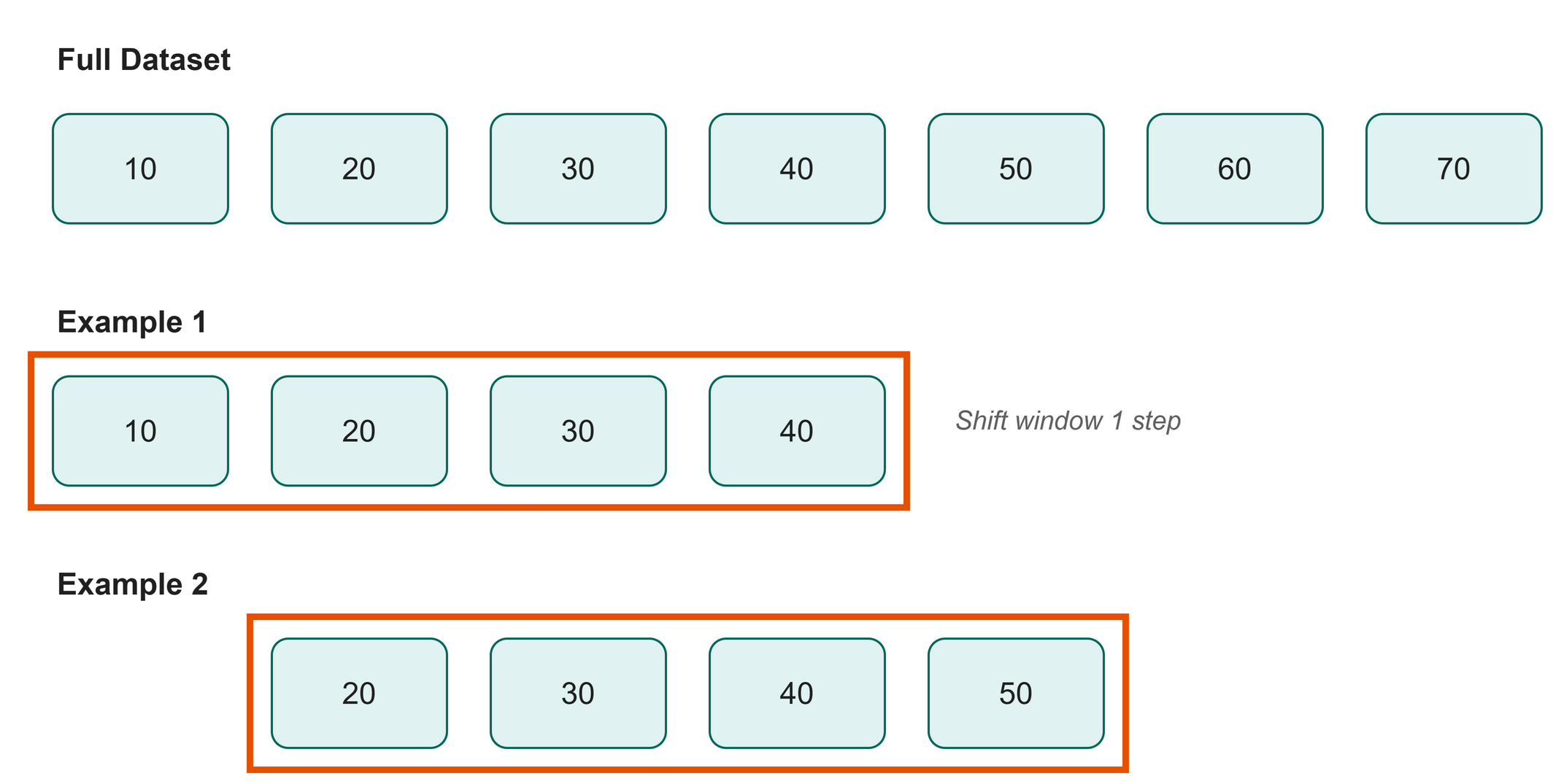A sliding window over text Figure 12.2: A sliding window creates multiple, overlapping examples from one long text.

Imagine a window that can only see a certain number of characters at a time. This is our block_size (the maximum context the model can handle). We place this window at the beginning of the text to grab our first sequence. Then, we slide the window one character to the right to grab our second sequence. We repeat this until we reach the end of the text.

Processing in Parallel: Batches¶

If we fed each sequence to the model one by one, training would crawl. Modern computers, especially GPUs, are fantastic at doing the same math on many pieces of data at once, and they are wasted on one sequence at a time.

How much does it matter? Rather than guess, time it:

Terminal

$ python src/examples/ch12_batch_speed.py
32 sequences, one at a time : 2.191 s
the same 32 as one batch    : 0.245 s
batching is 9.0x faster on this machine

Nine times faster, on an ordinary laptop with no GPU. The training run in Chapter 13 takes about six and a half minutes; one sequence at a time it would run closer to an hour. On a GPU, where thousands of arithmetic units sit idle waiting for work, the gap is wider still.

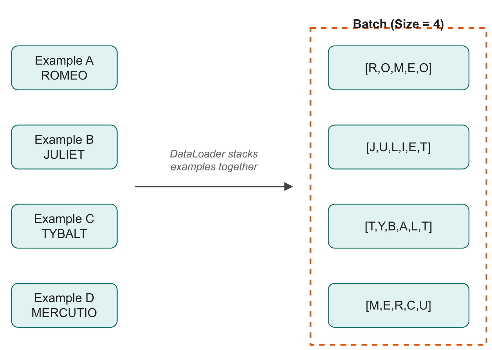Combining examples into a batch Figure 12.3: A batch stacks multiple independent examples into a single block.

We group multiple sequences together into a batch, as illustrated in Figure 12.3. If our batch size is 32, we pass 32 independent sequences through the model in one go. The model processes them in parallel, calculates the loss for all 32, and averages it out.

Why 32 and Not 1, or 1,000¶

Speed is only half the reason to batch. The other half is the quality of the step the model takes.

Remember what the loss is for: it produces a direction to nudge the weights. With a batch of 1, that direction comes from a single stretch of Shakespeare, which might happen to be a stage direction, a run of dialogue, or a line of mostly spaces. The model would lurch after each one, correcting hard for whatever it just saw. Averaging the loss over 32 independent sequences cancels most of that noise out, so each step points somewhere closer to the truth for the text as a whole.

Why not 1,000, then? Two reasons. The whole batch has to fit in memory at once, and memory is the limit you hit first on a laptop. Beyond that, the returns fade: averaging 1,000 sequences gives a direction only slightly truer than averaging 32, while each step costs thirty times as much. The number 32 is not sacred, and you will see other books use 16 or 64. It is simply a size that is large enough to steady the direction and small enough to fit.

This brings us to the start of the "Training" stage on our map. With our data batched and ready, we can finally feed it into the model and start the training loop.

Code¶

To handle this efficiently, we use two built-in PyTorch tools: Dataset and DataLoader (flow shown in Figure 12.4).

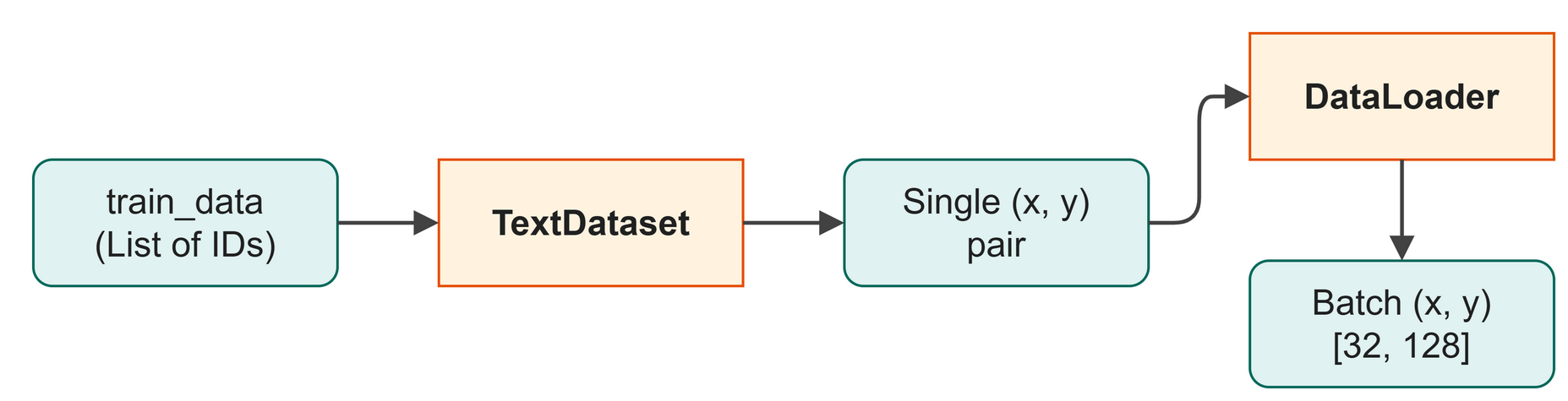Code flow: raw data into dataset and dataloader Figure 12.4: The Dataset handles the sliding window, and the DataLoader stacks the examples into a batch.

src/ch11_dataloader.py (excerpt)
class TextDataset(Dataset):
    def __init__(self, data, block_size):
        self.data = data
        self.block_size = block_size

    def __len__(self):
        # We need block_size + 1 tokens to form one (input, target) pair
        return len(self.data) - self.block_size

    def __getitem__(self, idx):
        # Input is a block of text
        x = self.data[idx     : idx + self.block_size]
        # Target is the same text, shifted one character to the right
        y = self.data[idx + 1 : idx + self.block_size + 1]
        return x, y

train_dataset = TextDataset(train_data, gpt_cfg.block_size)
val_dataset   = TextDataset(val_data,   gpt_cfg.block_size)

## DataLoader automatically batches the data for us
train_loader = DataLoader(
    train_dataset, batch_size=train_cfg.batch_size, shuffle=True
)

And how to run the full script:

Terminal

$ python src/ch11_dataloader.py
Data loaded: 1,115,394 total tokens
  Train : 1,003,854 tokens
  Val   : 111,540 tokens

Dataset sizes:
  Train examples: 1,003,726
  Val   examples: 111,412

DataLoader config:
  Batch size  : 32
  Train batches per epoch: 31,367

--- Inspecting one batch ---
x_batch shape: torch.Size([32, 128])  (batch_size, block_size)
y_batch shape: torch.Size([32, 128])  (batch_size, block_size)

First example in batch:
  x (input)  : 'ness! serious vanity!\nMis-shapen chaos of well-seeming for...
  y (target) : 'ess! serious vanity!\nMis-shapen chaos of well-seeming form...
  (y is x shifted by 1 character)

DataLoader ready! Ready for Chapter 13.

What just happened:

We loaded our text file and converted it to token IDs.
Lines 12 and 14 implement the sliding window logic in TextDataset, returning the sequence and its shifted target starting at idx.
Lines 21 to 23 create a DataLoader that automatically batches and shuffles the training data.
We grabbed one batch and inspected it to confirm the target y is just the input x shifted by one character.

Shape Check:

Table 12.1 lists the shapes of the batched input and target.

Table 12.1: Tensor shapes for the batched input and target sequences.

Variable	Shape	Meaning
`x_batch`	`[32, 128]`	32 sequences, each containing 128 input characters.
`y_batch`	`[32, 128]`	32 sequences, each containing 128 target characters.

Try It¶

We can see the sliding window in action with a tiny dataset.

src/examples/ch12_batching_demo.py
"""Show how a sliding window creates multiple overlapping examples."""
import torch

data = torch.tensor([10, 20, 30, 40, 50, 60, 70])
block_size = 3

print(f"Data: {data.tolist()}")
print(f"Block size: {block_size}\n")

## A simple loop to show the sliding window
for i in range(len(data) - block_size):
    x = data[i : i + block_size]
    y = data[i + 1 : i + block_size + 1]
    print(f"Example {i+1}:")
    print(f"  Input  : {x.tolist()}")
    print(f"  Target : {y.tolist()}")

Lines 12 and 13 slice the array to create overlapping sequences for the input and target.

Terminal

$ python src/examples/ch12_batching_demo.py
Data: [10, 20, 30, 40, 50, 60, 70]
Block size: 3

Example 1:
  Input  : [10, 20, 30]
  Target : [20, 30, 40]
Example 2:
  Input  : [20, 30, 40]
  Target : [30, 40, 50]
Example 3:
  Input  : [30, 40, 50]
  Target : [40, 50, 60]
Example 4:
  Input  : [40, 50, 60]
  Target : [50, 60, 70]

Try It

Open src/examples/ch12_batching_demo.py. Change block_size to 4 and run it again. Notice how the number of available examples decreases.

In Business

Imagine your house-style assistant needs to learn from a massive archive of 100,000 corporate documents. You wouldn't train it by showing it one word at a time. Processing data in parallel batches is like having the assistant review 32 different emails simultaneously, learning from all of them at once. It is the key to training efficiently at scale.

Watch Out

Be careful with the __len__ of your dataset. If you have 100 characters and a block_size of 10, you can only create 90 starting positions because you need 11 characters (10 for input, 1 extra for the target) for a valid example. That is why the code uses len(self.data) - self.block_size.

Key Takeaways¶

A sliding window extracts overlapping sequences from a continuous block of text.
Batching processes multiple independent sequences in parallel, dramatically speeding up training.
PyTorch's Dataset defines how to grab a single example.
PyTorch's DataLoader handles the tedious work of grouping examples into batches and shuffling them.

Check Your Understanding¶

If you have a sequence of 1000 tokens and a block size of 100, how many examples can a sliding window extract?
Why is batching important for training speed?
Why do we shuffle the training data?

Chapter 13: The Training Loop¶

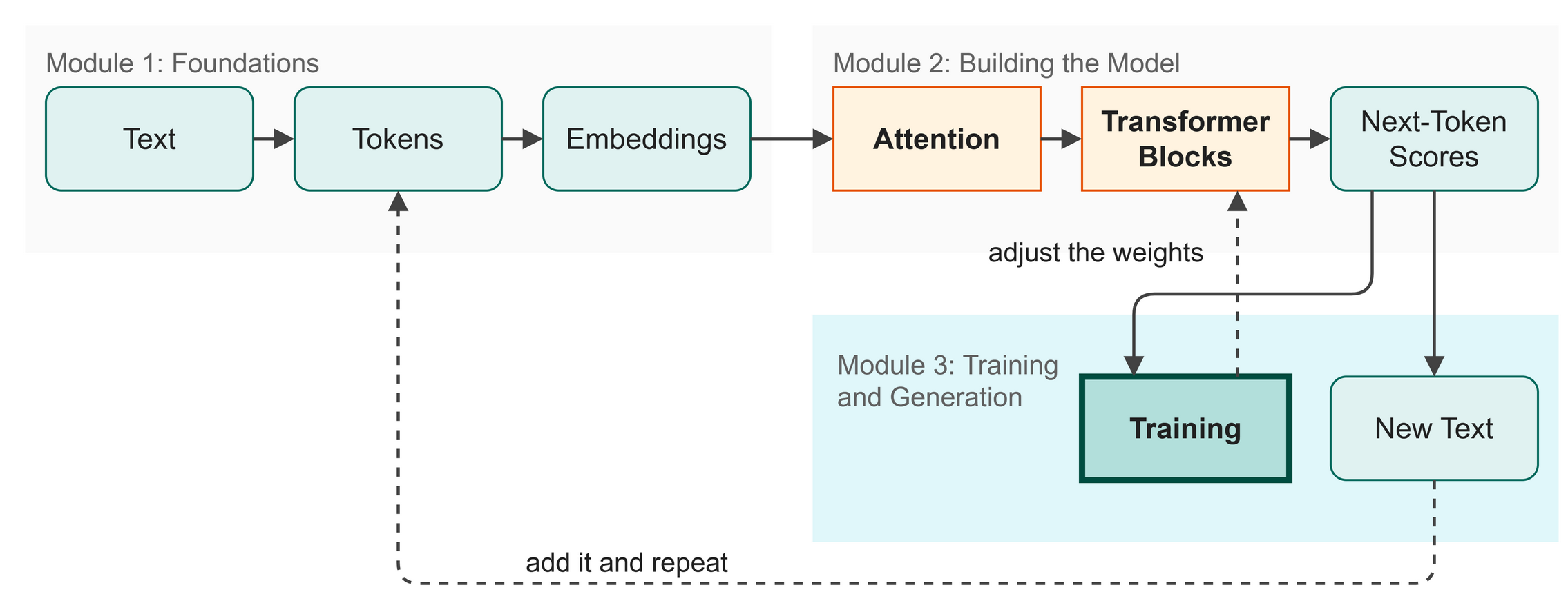You are here: Training Figure 13.1: The model makes predictions, measures its error, and adjusts its weights to improve.

Everything we have built so far comes down to this chapter. With our data batched and ready from Chapter 12, we have a model that can guess the next character, but right now, its guesses are no better than chance. In this chapter, we will write the loop that teaches it the patterns of the text it reads.

In this chapter you will:

Understand gradient descent as walking down a hill.
See what the learning rate does, by measuring three of them.
Build the four-step training loop.
Watch the model learn in real time, and read what its loss actually means.

Words to Know

Optimizer: The algorithm that updates the model's weights. We use Adam, a popular and steady choice.
Gradient: The direction we need to move our weights to increase the error. We move in the opposite direction to decrease it.
Backpropagation: The mathematical process of calculating the gradient for every single weight in the model.
Learning Rate: How far the optimizer moves the weights on each step. Too small and training crawls; too large and it can overshoot.

Theory¶

Walking Down the Hill¶

How does the model actually improve? Imagine you are blindfolded on a bumpy hillside, and you want to reach the very bottom (the lowest possible loss).

You can't see the whole hill, but you can feel the slope of the ground right under your feet. If the ground slopes up to your right, you know you should take a step to your left.

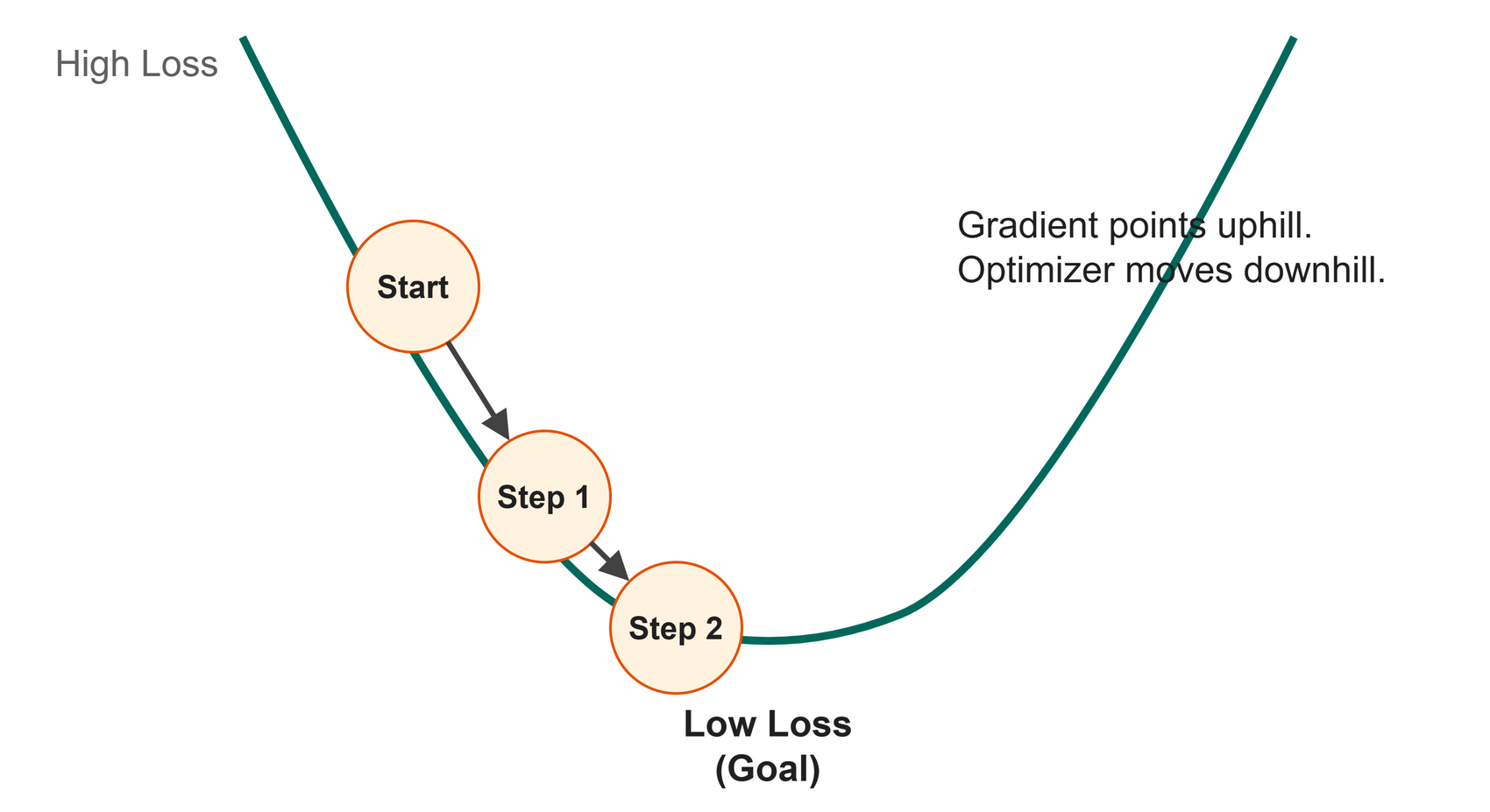Gradient descent as walking down a hill Figure 13.2: The optimizer takes small steps down the loss landscape to find the best weights.

This is gradient descent (Figure 13.2). The slope under your feet is the gradient (calculated by backpropagation). Taking a small step downhill is the optimizer updating the weights.

The Four-Step Loop¶

Training is a repetitive cycle that we run thousands of times (Figure 13.3):

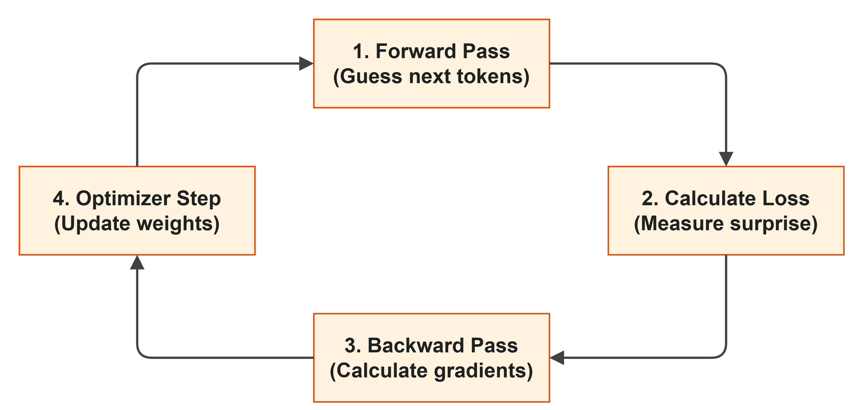The training loop cycle Figure 13.3: The four steps of the training loop.

Forward Pass: We pass a batch of data through the model to get its predictions.
Calculate Loss: We compare the predictions to the correct targets using cross-entropy.
Backward Pass: PyTorch's autograd engine automatically calculates the gradient for every weight in the model (loss.backward()).
Optimizer Step: The optimizer adjusts the weights slightly in the right direction (optimizer.step()).

How Big Should the Step Be?¶

Gradient descent tells you which way is downhill. It does not tell you how far to walk. That distance is the learning rate, and it is the one number beginners most often get wrong.

Our config sets it to 0.0003. Where does that come from? Rather than take it on faith, train the same model three times from the same starting weights, changing only the learning rate:

src/examples/ch13_learning_rate.py
for lr in (3e-3, 3e-4, 3e-5):
    torch.manual_seed(42)                       # same starting weights every time
    model = GPT(GPTConfig())
    optimizer = torch.optim.Adam(model.parameters(), lr=lr)

Terminal

$ python src/examples/ch13_learning_rate.py
lr=0.003    start 4.33  after 150 steps 2.35
lr=0.0003   start 4.33  after 150 steps 2.60
lr=3e-05    start 4.33  after 150 steps 3.31

The bottom row is the lesson most people need. At 0.00003 the steps are so small that after 150 steps the model has barely moved: 3.31, when random guessing is 4.17. It is learning, just far too slowly to be useful. If your loss is falling but crawling, suspect the learning rate before you suspect anything else.

The top row is more interesting, because it does not say what you might expect. Ten times the learning rate learned faster here, reaching 2.35 while our chosen rate reached 2.60. So why does the book not use it?

Because 150 steps is not 3,000. A large step size is a gamble: it covers ground quickly, and it can also overshoot the bottom of the valley and bounce, or blow up entirely. Our run of 150 steps is too short to show that either way, so we will not pretend it does. What we can say is that 0.0003 is the cautious choice, it reaches a loss of 1.74 over the full run, and it got there without drama. Trying 0.003 for all 3,000 steps is a genuinely interesting experiment, and one you now have everything you need to run.

The "Aha!" Moment: It Learned¶

When we start training, the loss is around 4.3. Remember from Chapter 11 that a completely random model guessing among 65 characters expects a loss of 4.17. At the start, the model is worse than random.

But as the loop runs, the numbers start to move.

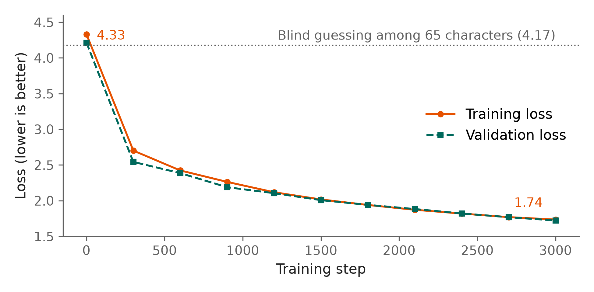Training loss dropping over time Figure 13.4: Over 3,000 steps, the model goes from blind guessing to predicting text with high confidence.

The loss plummets, as shown in Figure 13.4. By step 300, it is already at 2.7. By step 3,000, it reaches 1.74.

What the Loss Number Actually Means¶

A loss of 1.74 means nothing on its own. Here is how to read it.

Cross-entropy is the negative logarithm of the probability the model gave to the character that actually came next. Undo the logarithm and the probability comes back, which is a number you can reason about:

src/examples/ch13_loss_meaning.py
for name, loss in [("random guessing", math.log(VOCAB)),
                   ("step 1", 4.3280),
                   ("step 300", 2.7016),
                   ("step 3000", 1.7357)]:
    # Cross-entropy is the negative log of the probability given to the right answer
    prob = math.exp(-loss)
    print(f"{name:<16} loss {loss:.2f} -> {prob:6.1%} on the right character")

Terminal

$ python src/examples/ch13_loss_meaning.py
random guessing  loss 4.17 ->   1.5% on the right character
step 1           loss 4.33 ->   1.3% on the right character
step 300         loss 2.70 ->   6.7% on the right character
step 3000        loss 1.74 ->  17.6% on the right character

Now the numbers say something. At the start the model puts about 1.3% of its confidence on the correct character, slightly worse than the 1.5% you would get by drawing at random from 65 characters. Twelve times better than chance by the end sounds impressive, and it is. But read the absolute figure too: even fully trained, the model is wrong about the next character roughly four times in five.

Hold on to that, because it sets the right expectation for what you built. The model has learned which characters tend to follow which, how long words usually run, where the line breaks fall, and what a speaker's name looks like. It has not learned the rules of English, and it has certainly not learned to mean anything. You will see the evidence in Chapter 17, when it writes "Praviour soul to shall that that are the and not,": the shape of Shakespeare is there, the sense is not.

This completes the "Training" loop on our map. Our model is now a working engine that has learned the character patterns of its training data.

Code¶

Here is how simple the core loop is in PyTorch.

src/ch12_train.py (excerpt)
    optimizer = torch.optim.Adam(model.parameters(), lr=train_cfg.learning_rate)

    for step in range(1, train_cfg.max_iters + 1):
        x, y, train_iter = get_batch(train_loader, train_iter, device)

        # Forward pass
        logits = model(x)
        loss = F.cross_entropy(logits.view(-1, gpt_cfg.vocab_size), y.view(-1))

        # Backward pass
        optimizer.zero_grad()
        loss.backward()
        optimizer.step()

And how to run the full script:

Terminal

$ python src/ch12_train.py
Chapter 13: The Training Loop

Model parameters: 824,832
Training on     : cpu
Steps           : 3,000
Batch size      : 32
Block size      : 128

Starting training... (eval every 300 steps)
step     1/3000 | train loss: 4.3280 | val loss: 4.2114 | elapsed: 3s | ETA: 7595s
step   300/3000 | train loss: 2.7016 | val loss: 2.5433 | elapsed: 55s | ETA: 496s
...
step   900/3000 | train loss: 2.2633 | val loss: 2.1889 | elapsed: 160s | ETA: 372s
step  1200/3000 | train loss: 2.1185 | val loss: 2.1053 | elapsed: 210s | ETA: 314s
step  1500/3000 | train loss: 2.0174 | val loss: 2.0078 | elapsed: 248s | ETA: 248s

What just happened:

Line 1 creates an Adam optimizer to handle the weight updates.
Line 3 runs 3,000 steps of training, which takes about 20-30 minutes on a standard CPU laptop.
Lines 11 to 13 calculate the gradients and update the weights, driving the training loss down from 4.32 to 1.74.
We saved our hard-earned weights to a file so we can load them later.

Shape Check:

Table 13.1 lists the parameter count.

Table 13.1: Total adjustable parameters in the language model.

Variable	Shape	Meaning
`model.parameters()`	`824,832`	The total number of individual numbers (weights) the optimizer is adjusting.

Try It¶

We can see the mechanics of PyTorch's automatic gradients on a tiny scale.

src/examples/ch13_autograd_demo.py
"""Show how PyTorch automatically calculates gradients to update a weight."""
import torch

## A single weight starting at 2.0
weight = torch.tensor([2.0], requires_grad=True)

## Our simple 'model' multiplies input by weight
x = torch.tensor([3.0])
target = torch.tensor([12.0]) # We want output to be 12

print(f"Initial weight: {weight.item():.2f}")

for step in range(3):
    # Forward pass
    output = weight * x
    loss = (output - target) ** 2

    # Backward pass (calculate the gradient)
    loss.backward()

    print(f"Step {step+1}: Output={output.item():.2f}, "
          f"Loss={loss.item():.2f}, Gradient={weight.grad.item():.2f}")

    # Update weight (move in opposite direction of gradient)
    with torch.no_grad():
        weight -= 0.05 * weight.grad
        weight.grad.zero_()

print(f"Final weight: {weight.item():.2f}")

Lines 19, 26, and 27 show PyTorch computing the gradient and using it to adjust the weight toward the target.

Terminal

$ python src/examples/ch13_autograd_demo.py
Initial weight: 2.00
Step 1: Output=6.00, Loss=36.00, Gradient=-36.00
Step 2: Output=11.40, Loss=0.36, Gradient=-3.60
Step 3: Output=11.94, Loss=0.00, Gradient=-0.36
Final weight: 4.00

Try It

Open src/examples/ch13_autograd_demo.py. Change the starting weight to 10.0 and watch how the gradient pulls it down instead of pushing it up, always aiming for the target output of 12.

In Business

Training is where the real investment happens. When your company trains its house-style assistant, it pays for the compute time required to run this loop billions of times across thousands of documents. The loss curve is your main dashboard metric: as long as it is going down, the assistant is getting better at mimicking your corporate voice.

Watch Out

Never forget optimizer.zero_grad() before loss.backward(). PyTorch accumulates gradients by default (adds them up). If you don't zero them out at the start of the backward pass, your model will take steps based on a mix of the current batch and all previous batches, wandering off in the wrong direction.

Key Takeaways¶

Training is a loop of four steps: Forward, Loss, Backward, Step.
Gradient descent finds the lowest loss by taking small steps downhill.
We use the torch.optim.Adam optimizer to manage the complex math of updating the weights.
The model starts by guessing blindly (loss > 4.17), but over 3,000 steps, it learns the patterns of the text and the loss plummets.

Check Your Understanding¶

What are the four main steps inside the training loop?
What does loss.backward() actually do?
Why is a dropping loss curve a good sign?

Chapter 14: Checkpointing¶

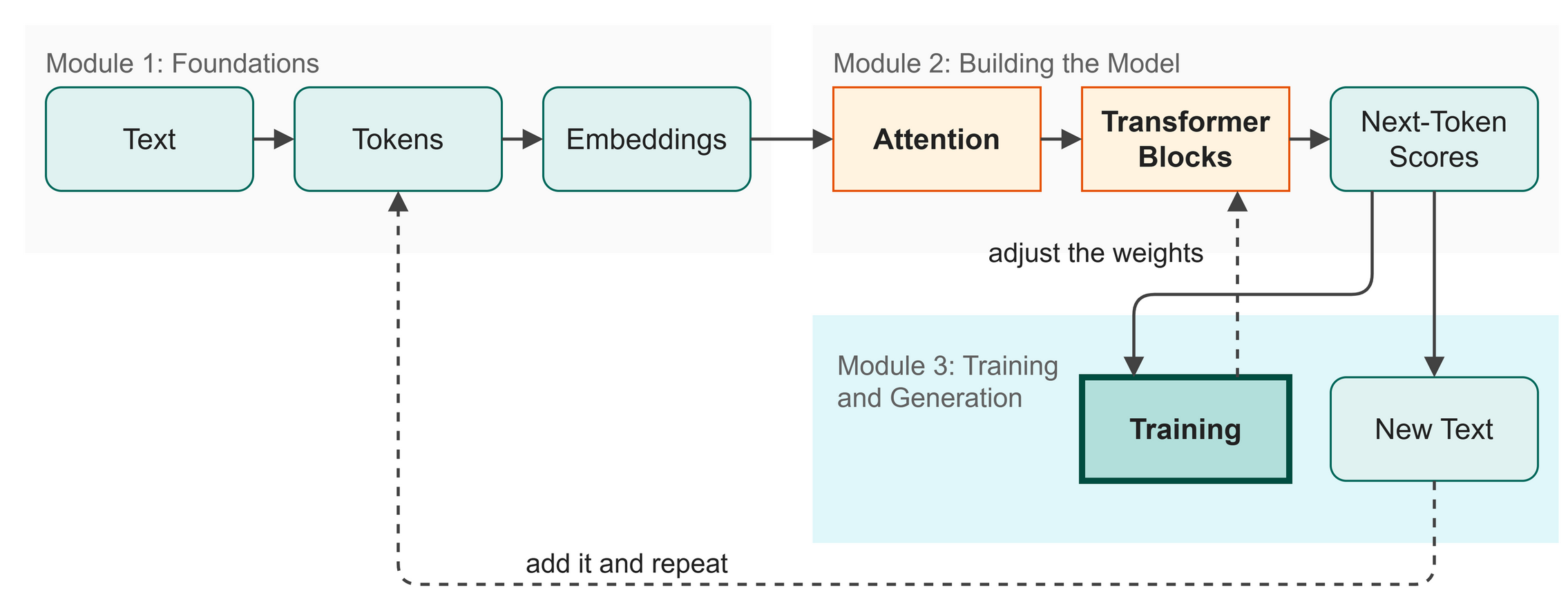You are here in the big picture Figure 14.1: Where we are: we have trained the model and now we save its weights.

Training a language model takes time. Once the model learns from the data, you need to save its knowledge so you can use it later without retraining. In this chapter you will:

Save a trained model to a file.
Load a saved model back into memory.
Switch the model from training mode to evaluation mode.

Words to Know

Checkpoint: a file containing the saved state (weights and configuration) of a model at a specific point in training.
State Dict: a PyTorch dictionary that maps each layer of the model to its learned weights.
Dropout: A technique that randomly turns off some neurons during training to prevent memorizing the data.

Theory¶

The Checkpoint File¶

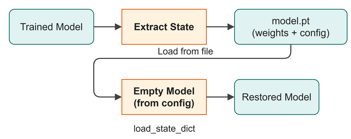A trained model saves its weights and configuration to model.pt; later, an empty model is built from the configuration and restored with the saved weights. Figure 14.2: The save and load round trip: the model's structure and its learned weights are both stored in the checkpoint.

A checkpoint is the model's save file. When you train a model, you adjust its weights (the parameters). These learned parameters are stored in a dictionary called a state_dict.

However, the weights alone are not enough. If you close your program and come back tomorrow, PyTorch will not know how many layers or attention heads your model has. To bring the model back to life, you must save both its configuration (the architecture skeleton) and its state dictionary (the learned weights). We also save the current training step and validation loss so we know how well the model performed.

Restoring the Model¶

Loading a checkpoint happens in three steps:

Load the saved dictionary from the file on disk.
Build an empty model using the saved configuration.
Pour the saved weights into the empty model.

Once the model is loaded, you must call model.eval(). During training, neural networks often use a technique called dropout, which randomly turns off some neurons to prevent the model from memorizing the data. Calling model.eval() turns off dropout, ensuring that all neurons are active and the model gives reliable, deterministic answers when generating text.

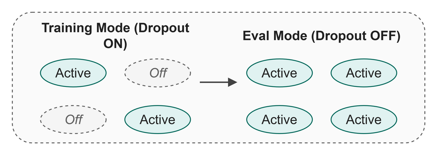Training mode with some neurons off versus eval mode with all neurons active Figure 14.3: In evaluation mode, all neurons are active and the model is ready to generate text deterministically.

As the "where we are" map shows, saving the checkpoint captures the model after the training loop, preparing it to generate new text in the final stage.

In Business

Think of our house-style assistant. The training process analyzed your company's archive to learn its voice. If the server restarts, you don't want to re-read the entire archive. A checkpoint saves that learned company voice to a tiny file that you can load instantly on any machine.

Code¶

We use the PyTorch torch.load() function to read our checkpoint file, and model.load_state_dict() to apply the weights.

src/ch13_checkpoint.py (excerpt)
    checkpoint = torch.load(
        CHECKPOINT_PATH, map_location="cpu", weights_only=False
    )
    step     = checkpoint["step"]
    val_loss = checkpoint["val_loss"]
    cfg      = checkpoint["gpt_cfg"]

    model = GPT(cfg)
    model.load_state_dict(checkpoint["model_state"])

    # Set to evaluation mode (disables dropout, making outputs deterministic)
    model.eval()

Let's see what happens when we load the checkpoint created at the end of the previous chapter.

Terminal

$ python src/ch13_checkpoint.py
--- 2. Load the checkpoint ---
Loading checkpoint from: checkpoints/model.pt
  Trained for  : 3000 steps
  Val loss     : 1.7228
  Model config : 4 layers, 128 embd, 4 heads

--- 3. Rebuild the model from the checkpoint ---

Model rebuilt successfully: 824,832 parameters loaded

--- 4. Verify the model works ---
Input shape : torch.Size([1, 10])
Output shape: torch.Size([1, 10, 65])   (looks good!)

--- 5. Show checkpoint file size ---

Checkpoint file size: 4.18 MB
(Small enough to share by email!)

Checkpointing done! Ready for Chapter 15.

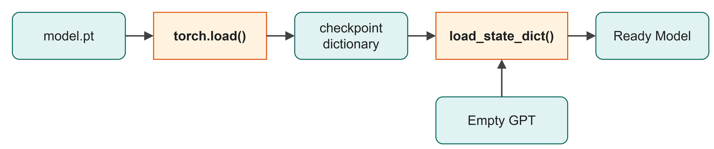Code flow: load file, extract dictionary, load into empty model Figure 14.4: How the checkpoint loading code flows: from file to ready model.

What just happened:

Line 1 loaded the checkpoint model.pt from disk.
Line 8 built an empty GPT model using the loaded configuration.
Line 9 populated the model with the 824,832 learned parameters.
Line 12 switched the model to evaluation mode.
We verified the checkpoint file is tiny (just over 4 megabytes).

Shape Check¶

Table 14.1 shows the tensor shapes when verifying the loaded model.

Table 14.1: Input and output shapes for the restored model.

Tensor	Shape	What it means
`dummy_ids`	`[1, 10]`	1 sequence of 10 token IDs.
`logits`	`[1, 10, 65]`	65 vocabulary scores for each of the 10 positions.

Try It¶

Try It

You can inspect the checkpoint directly by writing a small script to load the file.

src/examples/ch14_inspect_checkpoint.py (excerpt)
# ...
checkpoint_path = os.path.join(
    os.path.dirname(__file__), "..", "..", "checkpoints", "model.pt"
)
# ...
checkpoint = torch.load(
    checkpoint_path, map_location="cpu", weights_only=False
)
print("Keys in checkpoint:", list(checkpoint.keys()))
print("Training step:", checkpoint.get("step"))

Lines 9 and 10 print the keys and the training step from the loaded checkpoint dictionary.

Terminal

$ python src/examples/ch14_inspect_checkpoint.py
Keys in checkpoint: ['model_state', 'gpt_cfg', 'step', 'val_loss']
Training step: 3000

Key Takeaways¶

A checkpoint saves the model's configuration and learned weights to a file.
You rebuild the model by creating an empty network with the configuration, then loading the weights with load_state_dict.
Always call model.eval() after loading a model to turn off training features like dropout.
A model with 825,000 parameters takes up only about 4 MB of disk space.

Check Your Understanding¶

Why do we need to save the model's configuration in the checkpoint along with the weights?
What happens if you forget to call model.eval() before generating text?
What PyTorch function do we use to apply the saved weights to the newly built model?

Chapter 15: Greedy and Sampling¶

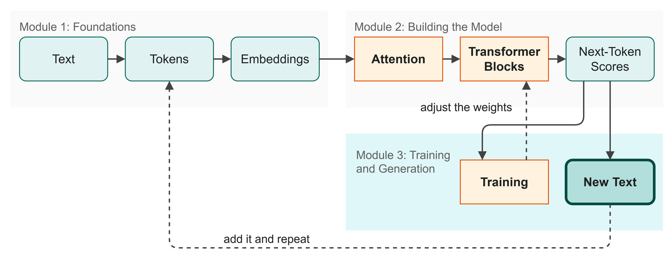You are here in the big picture Figure 15.1: Where we are: we are ready to generate new text using the trained model.

Our model is trained and loaded. Now we want to use it to generate new text. But the model doesn't just output a single character; it produces a list of 65 scores (logits), one for each possible character in the vocabulary. We need a strategy to pick the winner. In this chapter you will:

Generate text by always choosing the highest-scoring character (greedy decoding).
Generate text by choosing characters randomly based on their probabilities (sampling).
Compare the trade-offs between deterministic and creative text generation.

Words to Know

Greedy Decoding: always picking the single highest-probability token.
Sampling: choosing the next token randomly, giving higher-probability tokens a better chance to be selected.

Theory¶

Greedy Decoding¶

The simplest strategy is to always pick the character with the highest score. This is called greedy decoding.

While it seems logical to always pick the "best" answer, greedy decoding has a major flaw: it often gets stuck in loops. Imagine the model learns a common phrase. It predicts the next character, and that character becomes part of the context. The context looks familiar, so it predicts the next character of the phrase, and soon it is repeating the same phrase forever.

Greedy decoding is deterministic: if you give it the same prompt, it will always produce the exact same text.

Sampling¶

To avoid repetitive loops, we can use a strategy called sampling. Instead of automatically taking the top character, we turn the raw scores (logits) into percentages (probabilities) and draw a winner randomly.

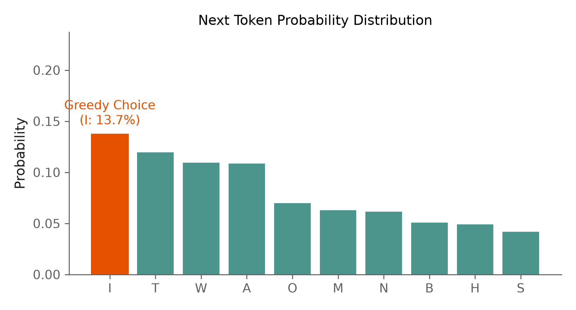Argmax taking the top peak vs sampling from the distribution Figure 15.2: Greedy decoding always takes the top peak; sampling draws randomly from the distribution.

If the letter "e" has a 60% probability, it will be chosen 60% of the time. If "x" has a 1% probability, it is rarely chosen, but it still has a chance. This introduces variety and breaks repetitive loops, making the text feel more natural and creative. However, it also means the output is unpredictable and changes every time you run it.

As shown on the "where we are" map, generation loops the New Text back to the Tokens step: the model predicts one character, we add it to the prompt, and the cycle repeats.

In Business

In our house-style assistant, the choice between greedy and sampling depends on the task. If the assistant is answering a factual question from a company manual, you want greedy decoding (safe, predictable, exact). If it is drafting a creative marketing email in the company voice, you want sampling (varied, creative, exploring new options).

Code¶

We implement both strategies in the same generation loop. The core difference is how next_id is chosen.

src/ch14_generate_greedy.py (excerpt)
def generate_greedy(model, prompt, encode, decode, cfg, max_new_tokens=200):
    # Always picks the token with the highest predicted score
    ids = torch.tensor([encode(prompt)], dtype=torch.long)
    for _ in range(max_new_tokens):
        ctx     = ids[:, -cfg.block_size:]
        logits  = model(ctx)
        next_id = logits[:, -1, :].argmax(dim=-1, keepdim=True)
        ids     = torch.cat([ids, next_id], dim=1)
    return decode(ids[0].tolist())

def generate_sample(model, prompt, encode, decode, cfg, max_new_tokens=200):
    # Picks the next token randomly based on the model's probabilities
    ids = torch.tensor([encode(prompt)], dtype=torch.long)
    for _ in range(max_new_tokens):
        ctx    = ids[:, -cfg.block_size:]
        logits = model(ctx)
        probs  = F.softmax(logits[:, -1, :], dim=-1)
        next_id = torch.multinomial(probs, num_samples=1)
        ids = torch.cat([ids, next_id], dim=1)
    return decode(ids[0].tolist())

Line 7 picks the character with the single highest score for greedy decoding. Lines 17 and 18 turn the scores into probabilities and draw a winner randomly for sampling.

Code flow: model(ctx) gives logits, argmax or multinomial picks next_id, which is appended to context Figure 15.3: The generation loop predicts one character at a time and appends it to the context.

Notice ids[:, -cfg.block_size:]. We crop the context to block_size tokens before passing it to the model. The model only learned to read a specific maximum length (our block size of 128) during training, so we must feed it at most that many tokens. We also take logits[:, -1, :] because we only care about the predictions for the very last character.

Let's see the two strategies in action with the prompt ROMEO:\n.

Terminal

$ python src/ch14_generate_greedy.py
--- GREEDY (always picks highest-score token) ---
ROMEO:
I will the come the some the stand the son,
And the so shall the see the shall the see the stand
...
--- SAMPLING (picks randomly from distribution) ---
ROMEO:
My must greather, but what it? whom, he ere.

EBRUTUS:
Morcy there bagainVain, I will ever may
To epated as great that the appral tankswain
...
--- Observations ---
Greedy tends to be more repetitive.
Sampling is more varied but can make unexpected choices.

Terminal

$ python diagrams/charts/ch15_probabilities.py
Saved chart: ch15-probabilities.png

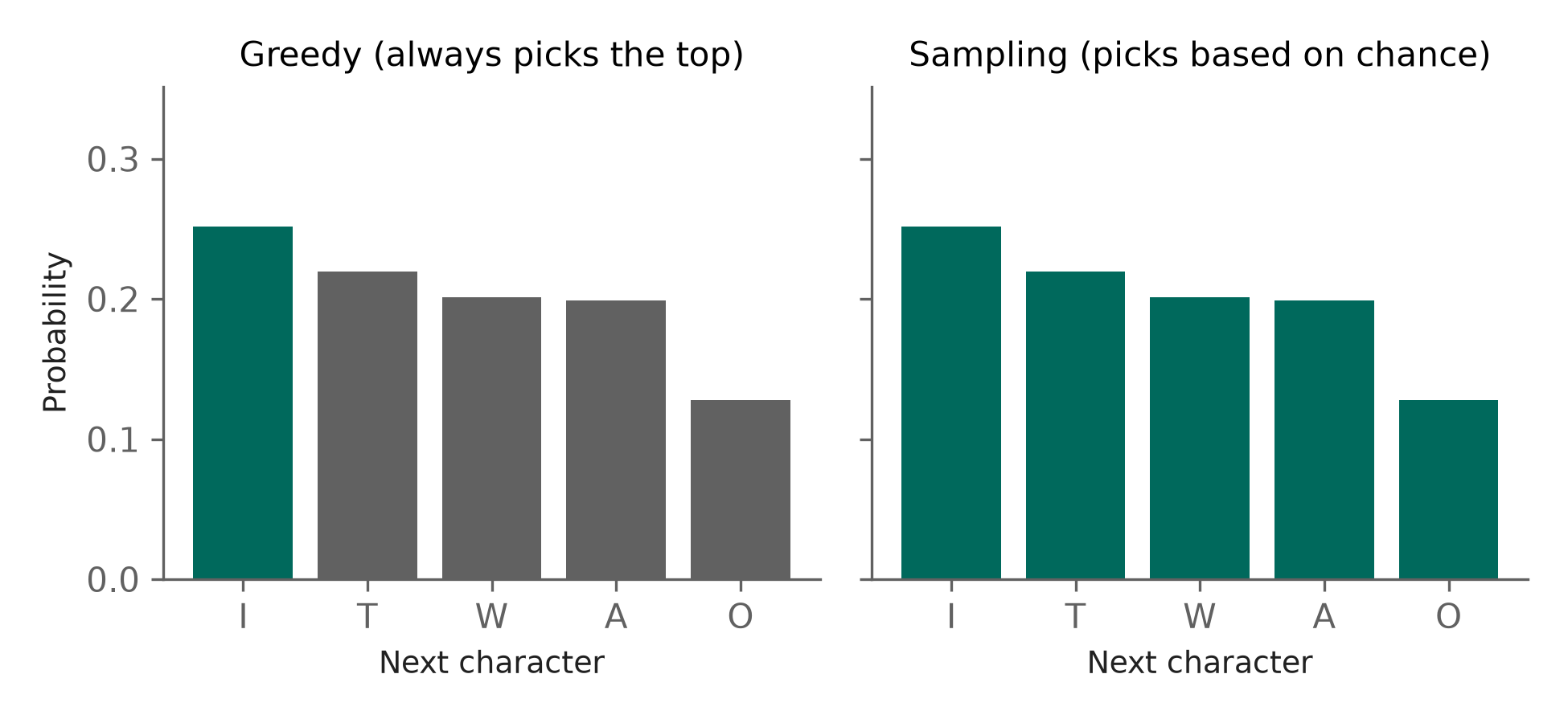Bars comparing greedy and sampling on the same probabilities Figure 15.4: Greedy always picks the tallest bar; sampling can pick any bar based on its height.

What just happened:

The greedy approach quickly got stuck in a repetitive loop ("the shall the shall...").
The sampling approach produced varied, non-repetitive text, but it included some strange spellings ("greather", "bagainVain") because it occasionally picked low-probability characters.

Shape Check¶

Table 15.1 details the shapes used during the character prediction step.

Table 15.1: Tensors used during the text generation loop.

Tensor	Shape	What it means
`logits[:, -1, :]`	`[1, 65]`	65 vocabulary scores for the final character in the sequence.
`next_id`	`[1, 1]`	1 chosen character ID.

Try It¶

Try It

Different starting prompts create different context for the model. Let's see how sampling handles new prompts.

src/examples/ch15_different_prompts.py (excerpt)
# ...
encode_fn = lambda s: encode(s, char_to_id)
decode_fn = lambda ids: decode(ids, id_to_char)

print(f"--- Prompt: 'KING:\\n' ---")
print(generate_sample(model, "KING:\n", encode_fn, decode_fn, cfg, 50))

print(f"\n--- Prompt: 'JULIET:\\n' ---")
print(generate_sample(model, "JULIET:\n", encode_fn, decode_fn, cfg, 50))

Lines 6 and 9 generate new text starting from two completely different prompts.

Terminal

$ python src/examples/ch15_different_prompts.py
--- Prompt: 'KING:\n' ---
KING:
My mine gore to kink on Villence,
For my love grin

--- Prompt: 'JULIET:\n' ---
JULIET:
What reason this bagainVain, I will evers,
As do p

Key Takeaways¶

Greedy decoding always chooses the highest-scoring token, which leads to predictable but highly repetitive text.
Sampling chooses the next token randomly based on the probability distribution, creating varied and natural text.
The generation loop works by predicting one character, appending it to the context, and repeating the process.
We crop the input context to the model's maximum block_size before each prediction.

Check Your Understanding¶

Why does greedy decoding often get stuck repeating the same phrase?
What PyTorch function do we use to randomly pick a token based on its probabilities?
Why do we slice the logits tensor with [:, -1, :] in the generation loop?

Chapter 16: Temperature and Top-k¶

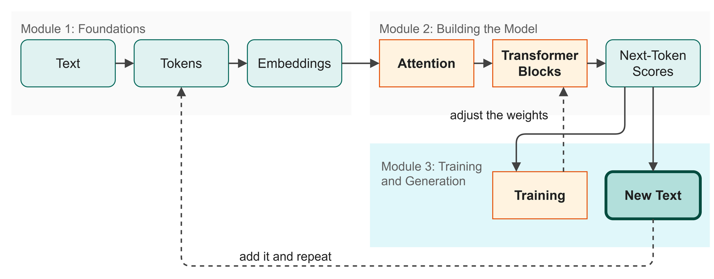You are here in the big picture Figure 16.1: Where we are: we are tuning the text generation process.

Plain sampling gives us varied output, but it can be unpredictable. Sometimes the model chooses a very rare character that completely breaks the grammar or creates a nonsense word. We need controls to balance creativity with coherence. In this chapter you will:

Use temperature to adjust how risky the model's choices are.
Use top-k truncation to prevent the model from picking truly bad characters.
Combine these controls for optimal text generation.

Words to Know

Temperature: a number that scales the logits before they are turned into probabilities, controlling the randomness of the output.
Top-k: a limit that restricts the model to only sample from the k most likely next tokens, ignoring all others.

Theory¶

Two controls sit between the raw scores the model produces and the character it finally picks. Temperature reshapes the odds. Top-k decides which characters are allowed to compete at all. They are independent, and in practice you set both.

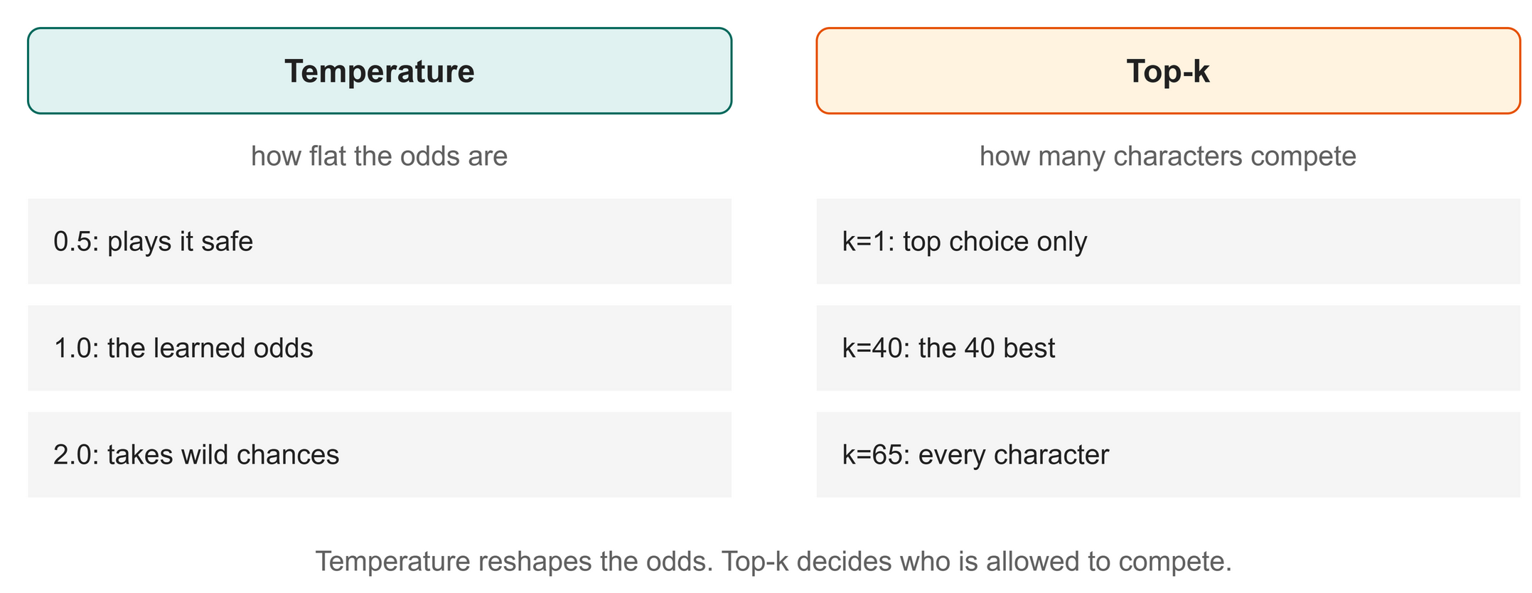The two generation controls side by side Figure 16.2: Temperature changes the shape of the odds; top-k changes how many characters stay in the running.

Temperature¶

Temperature is a simple math trick applied to the logits before the softmax step. By dividing all the raw scores by a number (the temperature), we change the shape of the probability distribution.

Terminal

$ python src/examples/ch16_temperature.py
Saved chart: ch16_temperature.png

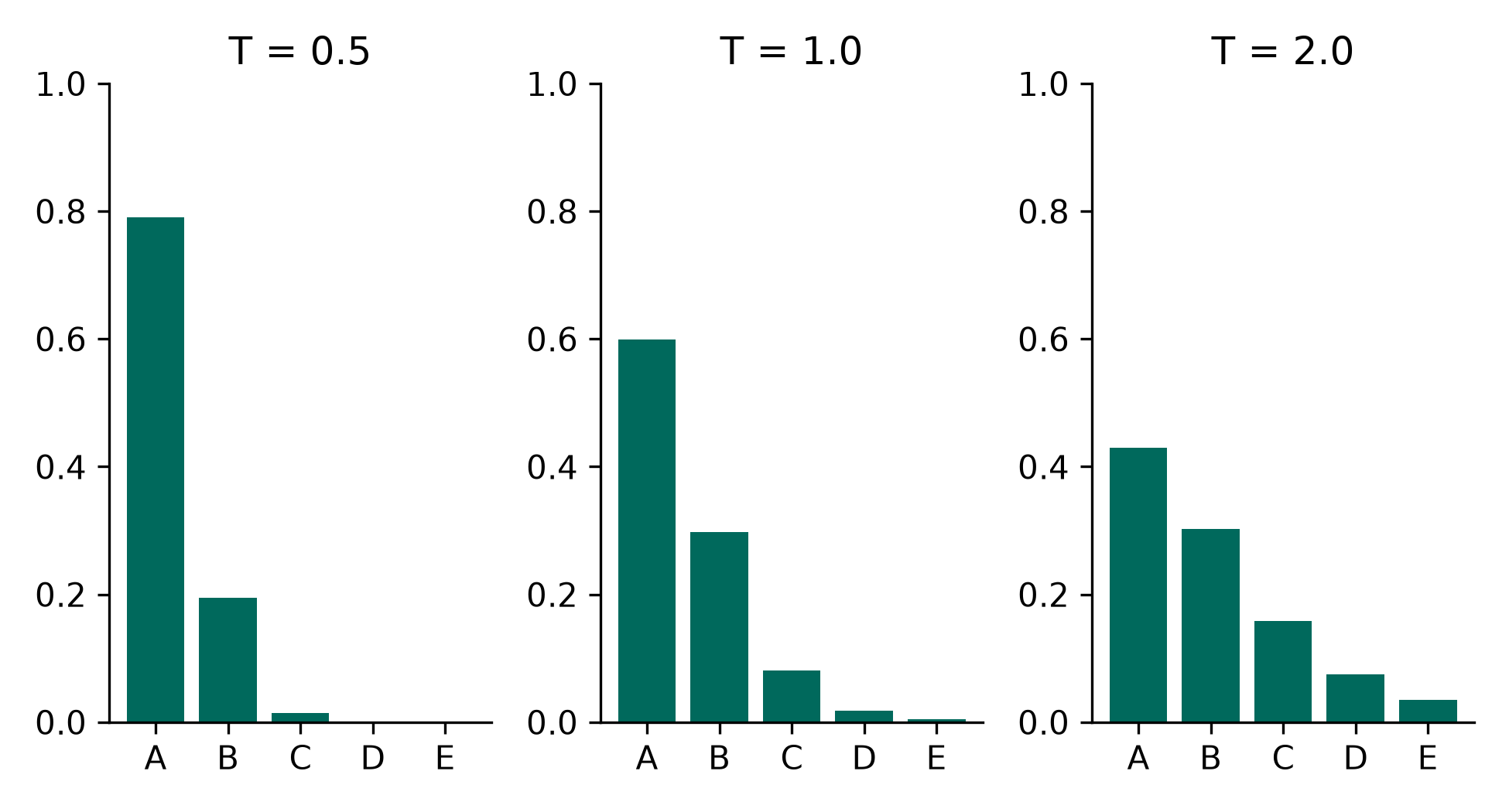Bars of next-character probabilities at three temperatures Figure 16.3: A plotted chart showing probabilities: low temperature sharpens the choice, high temperature flattens it.

Low temperature (e.g., 0.5): Dividing by a fraction mathematically stretches the scores apart. The top choice becomes overwhelmingly favored. The model plays it safe.
High temperature (e.g., 2.0): Dividing by a large number mathematically squishes the scores together. The probabilities flatten out, meaning unusual choices become more likely. The model takes risks.
T = 1.0: This is standard sampling. The model uses its learned probabilities exactly as they are.

Top-k¶

Even at a safe temperature, there is a tiny mathematical chance (say, 0.001%) that the model might pick a completely absurd character. If you generate 200 characters, those tiny chances add up, and a mistake is likely.

Top-k sampling solves this by putting a hard limit on the choices. If top_k = 40, we look at the 65 possible characters, keep the 40 with the highest scores, and completely discard the bottom 25 by setting their probabilities to zero. This cuts off the "long tail" of bad choices, guaranteeing that the model only samples from the most reasonable options.

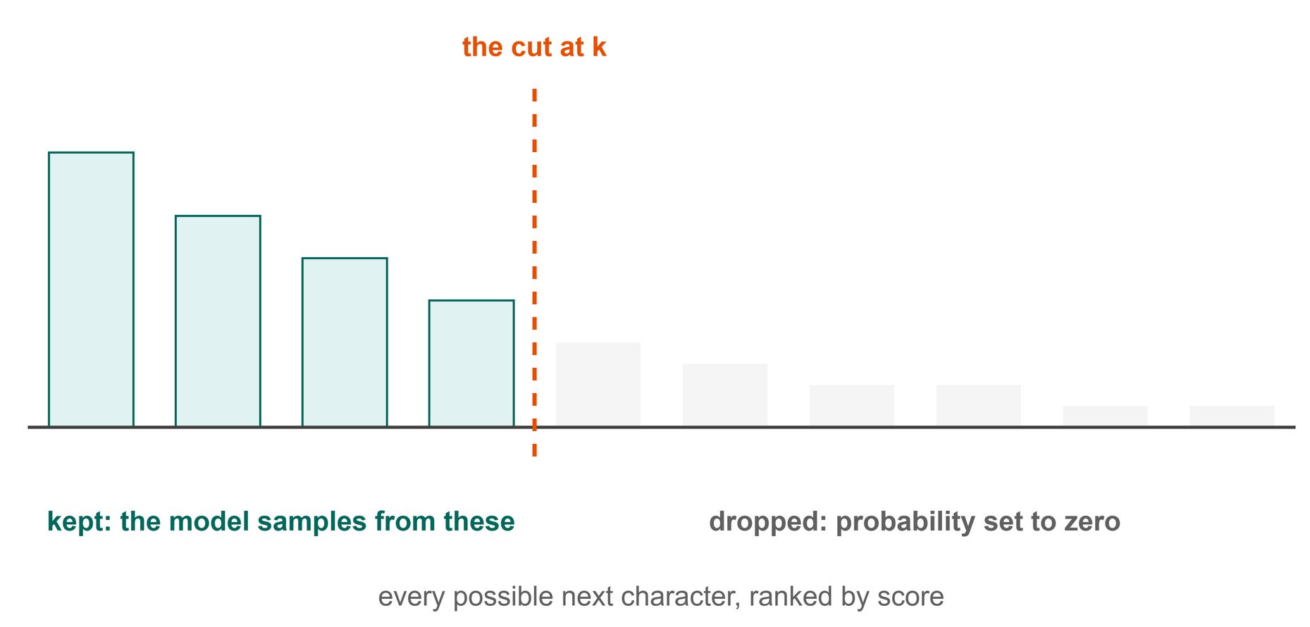Ranked scores with the low-scoring tail greyed out Figure 16.4: Top-k keeps the highest-scoring characters and zeroes the rest. Drawn here with ten characters and k = 4; the book's code uses 65 and k = 40.

As the "where we are" map shows, these controls adjust the Next-Token Scores right before generation loops back to produce the New Text.

In Business

For the house-style assistant, you might use a low temperature (0.5) when generating compliance documentation to ensure it stays close to the safest boilerplate text. When brainstorming marketing slogans, a higher temperature (0.9) with top-k sampling (40) will produce creative, surprising slogans that still make grammatical sense.

Code¶

We apply temperature and top-k right before the softmax function in the generation loop.

src/ch15_generate_sampling.py (excerpt)
        # Temperature controls randomness: lower is less random
        logits = logits / temperature

        # Top-k sampling limits the choices to the k most likely tokens
        if top_k is not None:
            threshold = logits.topk(top_k).values[:, -1, None]
            logits = logits.masked_fill(logits < threshold, float("-inf"))

        probs   = F.softmax(logits, dim=-1)
        next_id = torch.multinomial(probs, num_samples=1)

Line 2 divides the scores by the temperature to adjust randomness. Line 7 discards any score below the top-k threshold by setting it to negative infinity.

Code flow: logits divided by temperature, filtered by top-k, then softmaxed Figure 16.5: The code flow applies temperature first, then top-k, and finally softmax.

In PyTorch, we use masked_fill to apply top-k. We find the score of the 40th best token (threshold), and any token with a score lower than that gets its value changed to negative infinity (-inf). When softmax calculates probabilities, anything with a score of -inf mathematically becomes exactly 0.

Let's see how different settings affect the generated text.

Terminal

$ python src/ch15_generate_sampling.py
--- temp=0.5, top_k=40 ---
JULIET:
My must grace prove a son the come on my lord.

...
--- temp=0.8, top_k=40 ---
JULIET:
That will, my call thee for thee king win a be parder
The his in suppy ascented a not a say?
...
--- temp=1.0, top_k=40 ---
JULIET:
Look, do indo witned me devise thy grohed:
A give gring brothe whith ighers paison:
...
--- temp=1.5, top_k=40 ---
JULIET:
fattlyals give niet, thou stain, viful-wid thel,
Brob dayse mernion shing you fea,
...
--- temp=1.0, no top_k ---
JULIET:
Than mide smear of thou I am go vious, you me
now you scalf them frate ell, to 'till will she
...
--- Sweet spot ---
temperature=0.8 to 1.0 and top_k=40 usually gives the best results.

What just happened:

At temp=0.5, the text is coherent but relies heavily on common, safe words.
At temp=0.8 to 1.0, the text feels more natural and varied.
At temp=1.5, the text quickly devolves into chaos and made-up words ("fattlyals").
The sweet spot is typically a temperature between 0.8 and 1.0, combined with top_k=40.

Shape Check¶

Table 16.1 outlines the shapes of tensors used during top-k filtering.

Table 16.1: Tensors modified during the top-k sampling process.

Tensor	Shape	What it means
`threshold`	`[1, 1]`	The cutoff score (the 40th highest value).
`logits`	`[1, 65]`	65 scores, where 25 of them have been set to `-inf`.

Try It¶

Try It

Open the existing script src/examples/ch16_explore_temp.py and run it. It uses a very low temperature (0.1). You will notice it behaves almost exactly like greedy decoding, picking the safe top character every time!

Terminal

$ python src/examples/ch16_explore_temp.py
--- Prompt: 'JULIET:\n' ---
Generating with T=0.1...
JULIET:
I will the shall the shall be the son th...

Key Takeaways¶

Temperature adjusts the spread of the probabilities. Low temperature makes the model conservative, while high temperature makes it creative and risky.
Top-k restricts the model from ever picking the worst-scoring tokens, preventing bizarre errors.
To combine them, first apply temperature, then apply top-k to filter out the bad options, and finally convert to probabilities with softmax.
A combination of temperature=0.8 and top_k=40 is a widely used default for high-quality text generation.

Check Your Understanding¶

If you set the temperature to 0.1, what happens to the gap between the highest and lowest scores?
Why do we replace the eliminated scores in top-k with negative infinity (-inf) instead of 0?
Which step must happen first in the code: applying top-k or calculating softmax probabilities?

Chapter 17: Putting It All Together¶

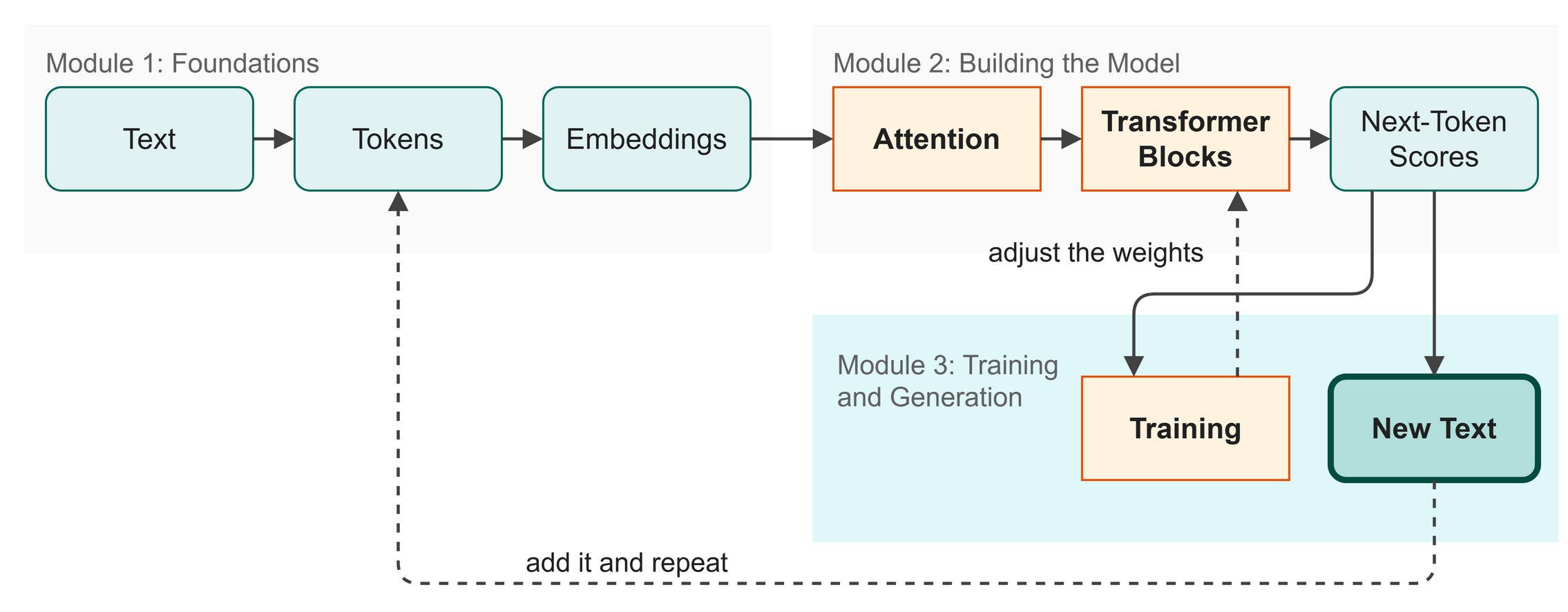You are here in the big picture Figure 17.1: Where we are: completing the full pipeline from text to language model.

You have built a language model from zero. Step by step, you wrote the code to tokenize text, embed it into vectors, apply self-attention, stack transformer blocks, train the weights using gradient descent, and generate new text with temperature and top-k sampling. In this final chapter you will:

Run the complete end-to-end pipeline in a single script.
See the full architecture in action.
Understand how your model relates to modern, production-grade LLMs.

Words to Know

End to End: a process that takes raw input (text) and goes through every necessary step to produce the final output (a trained model and generated text) without manual intervention.
Instruction tuning: A post-training step that teaches the model to answer questions and follow instructions.
RLHF: Reinforcement Learning from Human Feedback, a method to train models to behave politely and align with human preferences.

Theory¶

The Full Architecture¶

Take a look back at everything you built. This is not a "toy" architecture. You just wrote the exact same building blocks used by GPT-2, which is the architectural foundation of GPT-3, GPT-4, and many other modern Large Language Models (LLMs).

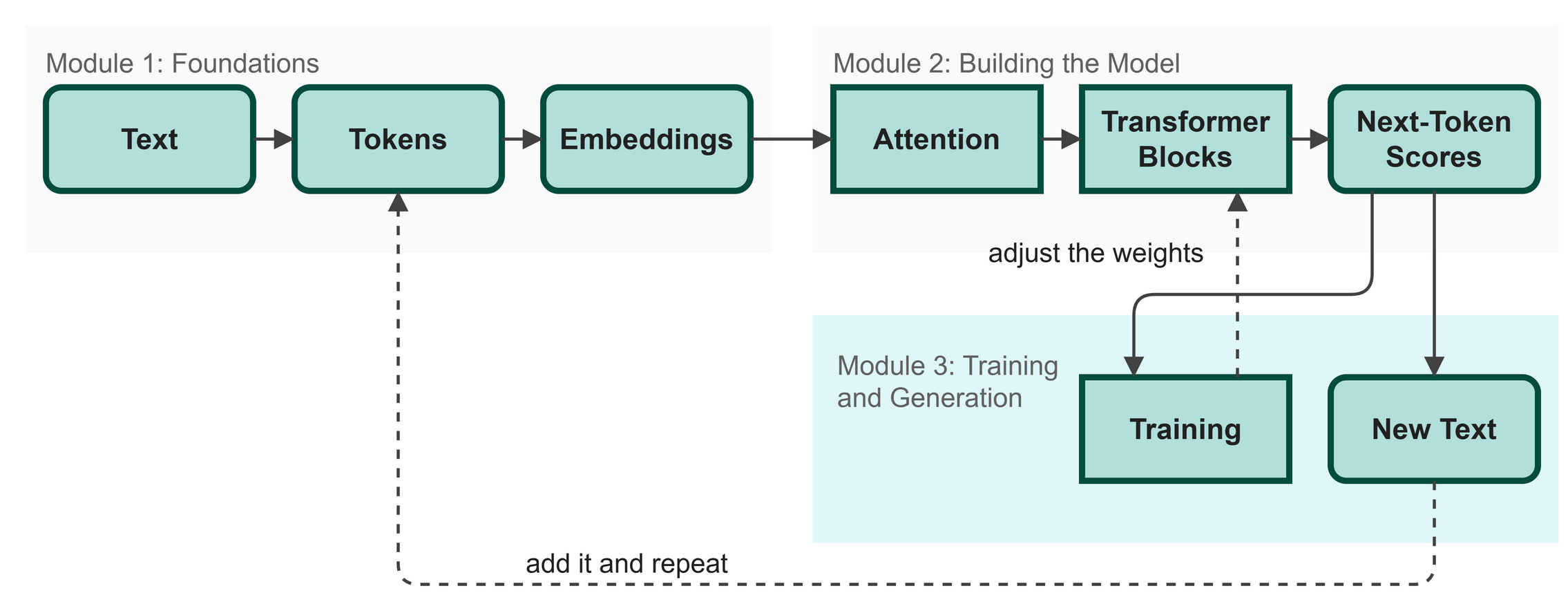The final full system map Figure 17.2: The complete system: from raw text to a trained language model.

The differences between your model and a massive production model are mostly a matter of scale:

Vocabularies: We used 65 characters; they use 50,000+ subword tokens.
Dimensions: We used a 128-dimensional embedding and 4 layers; they use thousands of dimensions and nearly a hundred layers.
Data: We trained on 1 megabyte of Shakespeare; they train on terabytes of internet text.
Hardware: We trained for a few minutes on a CPU; they train for months on thousands of specialized GPUs.

How Real Models Differ¶

While the fundamental transformer architecture (embeddings, attention, blocks, training) remains the same, modern models add refinements to optimize performance:

Instead of simple position lookups, they might use Rotary Positional Embeddings, which help models understand relative distances between words better.
Instead of standard multi-head attention, they might use Grouped-Query Attention, which saves memory and speeds up text generation.
After pretraining (what we did), they undergo Instruction Tuning and RLHF (Reinforcement Learning from Human Feedback) to learn how to answer questions politely rather than just predicting the next word.

As the "where we are" map shows, the end-to-end pipeline connects every stage from text ingestion to generation, wrapping the entire system into one continuous flow.

In Business

For our house-style assistant, this end-to-end script represents the full product lifecycle. In a business environment, you run this pipeline whenever the company archive changes: training a new model overnight on updated documents, validating it, and deploying the new checkpoint to serve your marketing and compliance teams.

Code¶

We have combined every piece of code from the previous chapters into one master script. It downloads the data, tokenizes it, creates the DataLoaders, builds the 825,000-parameter model, trains it for 3,000 steps, saves a checkpoint, and generates a sample text.

Code flow: Raw Text -> Tokenize -> Train Model -> Save .pt -> Generate Figure 17.3: The full script executes every step in sequence without manual intervention.

Let's run the smoke test.

Terminal

$ python src/ch16_full_pipeline.py
[1/7] Downloading dataset...
...
[2/7] Tokenizing...
...
[3/7] Creating DataLoaders...
...
[4/7] Building model...
...
[5/7] Training for 3000 steps...
...
step     1 | train: 4.2726 | val: 4.1660 | elapsed: 2s | ETA: 6148s
...
step  3000 | train: 1.7323 | val: 1.7411 | elapsed: 474s | ETA: 0s
...
[6/7] Saving checkpoint...
...
[7/7] Generating text...
...
GENERATED TEXT (temperature=0.8, top_k=40):
...
ROMEO:
Praviour soul to shall that that are the and not,

What just happened:

The model trained successfully and loss steadily decreased.
It generated brand new, Shakespeare-like text based on the patterns it learned.
While it makes some logical or grammatical mistakes, the character names, sentence structures, and vocabulary strongly mimic the training data.

Terminal

$ python diagrams/charts/ch17_generated_text.py
Saved chart: ch17-generated-text.png

Generated Shakespeare text rendered as an image Figure 17.4: The model generates new text.

Shape Check¶

Table 17.1 summarizes the parameter count of the fully assembled network.

Table 17.1: Final parameter count of the completed model.

Tensor	Shape	What it means
`model parameters`	`824,832`	The total number of weights the model learned during training.

Try It¶

Try It

Try testing the final model like a deployed production service. Create a script to load model_final.pt and respond to a user prompt.

src/examples/ch17_deploy.py (excerpt)
# ...
checkpoint_path = os.path.join(
    os.path.dirname(__file__), "..", "..", "checkpoints", "model_final.pt"
)

if not os.path.exists(checkpoint_path):
    # Fall back to model.pt if model_final.pt does not exist
    checkpoint_path = os.path.join(
        os.path.dirname(__file__), "..", "..", "checkpoints", "model.pt"
    )

checkpoint = torch.load(
    checkpoint_path, map_location="cpu", weights_only=False
)
# ...

Lines 6 and 8 check if the final checkpoint exists and fall back to a previous save if it doesn't.

Terminal

$ python src/examples/ch17_deploy.py
--- Prompt: 'USER: What is the news?\n' ---
USER: What is the news?

FROKENTER:
And with is there?

GLOUCEMIO:
All But, there come from the prainion; and every,
As do p

Key Takeaways¶

You successfully built the complete GPT architecture from scratch.
The fundamental components (tokenization, embeddings, self-attention, transformer blocks, and gradient descent) are the core of all modern LLMs.
Larger models mostly scale up these exact same components with more data, more parameters, and better hardware.
Refinements like RLHF and instruction tuning are applied after this pretraining process.

Check Your Understanding¶

What is the difference between the model we built and GPT-2?
Why does the model output sometimes contain spelling or logic errors despite being fully trained?
What is the purpose of an end-to-end pipeline in a business setting?

Glossary¶

Every term the book defines, in alphabetical order, with a plain definition and the chapter where it is first explained.

Table A.1: Glossary of terms used in this book.

Term	Meaning	Chapter
Autoregressive	Using your past outputs as inputs for your next step.	2
Backpropagation	The mathematical process of calculating the gradient for every single weight in the model.	13
Batching	Grouping multiple training examples together and processing them at the same time.	12
Block Size	The maximum number of tokens the model can look at at one time (its context window).	12
Causal Mask	A filter that prevents tokens from seeing future tokens.	6
Checkpoint	A file containing the saved state (weights and configuration) of a model at a specific point in training.	14
Concatenation	Joining multiple vectors end-to-end to form a longer vector.	7
Cross-Entropy Loss	A mathematical way to measure how wrong the model's predictions are. Lower is better.	11
DataLoader	A PyTorch utility that automatically groups individual examples into batches and shuffles them.	12
Dataset	A PyTorch class that defines how to retrieve a single training example.	12
Dropout	A technique that randomly turns off some neurons during training to prevent memorizing the data.	14
Embedding	A lookup table that maps a token ID to its vector.	5
End to End	A process that takes raw input (text) and goes through every necessary step to produce the final output (a trained model and generated text) without manual intervention.	17
Feed-Forward	A small neural network that processes each token independently.	8
GELU	A smooth curve that replaces negative numbers with near-zero values.	8
Gradient	The direction we need to move our weights to increase the error. We move in the opposite direction to decrease it.	13
Greedy Decoding	Always picking the single highest-probability token.	15
Instruction tuning	A post-training step that teaches the model to answer questions and follow instructions.	17
Key (K)	A vector representing what a token contains.	6
Language Model	A system that predicts the next token in a sequence.	2
LayerNorm	A step that resets numbers to a safe size so training stays stable.	8
LM Head	The final linear layer that maps internal numbers back to vocabulary words.	10
Logits	The raw scores the model outputs for each possible next token.	10
Matrix Multiplication	Combining two tensors to transform data.	3
Multi-Head Attention	Running several attention operations simultaneously.	7
Optimizer	The algorithm that updates the model's weights. We use Adam, a popular and steady choice.	13
Package Manager	A tool that downloads and installs code libraries.	1
Parameters	The numbers inside the model that adjust during training.	2
Projection	A linear layer that blends the concatenated outputs.	7
PyTorch	A library for doing math on large arrays of numbers very quickly.	3
Query (Q)	A vector representing what a token is looking for.	6
Repository	A folder of code stored online.	1
Residual Connection	A shortcut that lets information skip a step, keeping the original signal intact.	9
RLHF	Reinforcement Learning from Human Feedback, a method to train models to behave politely and align with human preferences.	17
Sampling	Choosing the next token randomly, giving higher-probability tokens a better chance to be selected.	15
Self-Attention	A mechanism where tokens evaluate every other token in the sequence to gather context.	6
Shape	The dimensions of a tensor (like rows and columns).	3
Softmax	A function that turns any numbers into probabilities that sum to 1.	3
State Dict	A PyTorch dictionary that maps each layer of the model to its learned weights.	14
Temperature	A number that scales the logits before they are turned into probabilities, controlling the randomness of the output.	16
Tensor	A multi-dimensional array of numbers.	3
Terminal	A text-based window where you type commands.	1
Token	One small piece of text, here a single character.	2
Tokenizer	A function that turns text into tokens and then into numbers.	4
Top-k	A limit that restricts the model to only sample from the k most likely next tokens, ignoring all others.	16
Transformer Block	A reusable block of code containing attention, feed-forward, and normalization.	9
Value (V)	A vector holding the actual information to be shared.	6
Vector	A list of numbers that acts as a coordinate in a high-dimensional space.	5
Virtual Environment	An isolated toolbox for a single project's packages.	1

Ten Papers That Built Generative AI¶

Every idea in this book was somebody's result first. These ten papers are the ones the rest stands on: each solved a problem that was blocking the field, and each changed what people built afterwards. They are in the order the story runs, from how a network learns at all to how a text predictor became something you can give instructions to.

You do not need the mathematics to follow them. Each entry says what was not working, what the paper did about it, and why it still matters, and then gives the reference so you can read the original. All ten are free to read.

Table B.1: The ten papers, in the order the ideas arrived.

#	Paper	Year	What it settled
1	Backpropagation	1986	Gave every weight in a deep network its share of the blame.
2	Long short-term memory	1997	Gave a sequence model a memory it could keep over long text.
3	Word vectors	2013	Turned word meaning into distance in a vector space.
4	Attention	2014	Let a model look back over its input and weigh what mattered.
5	The Transformer	2017	Kept attention, removed the step-by-step reading.
6	Pre-training and transfer	2018	Trained one model on plain text, then reused it everywhere.
7	Decoder-only language models	2019	Showed next-token prediction alone learns many tasks.
8	Scaling laws	2020	Made the pay-off from more data and compute predictable.
9	Few-shot prompting	2020	Taught a model a task from examples in the prompt.
10	Learning from human feedback	2022	Turned a text predictor into something that follows instructions.

Backpropagation (1986)¶

How a network learns anything at all. A network with layers in the middle had an obvious problem: when the answer came out wrong, nobody could say which of the middle weights was at fault. This paper gave the answer. Send the error backwards through the network and give each weight a share of the blame in proportion to how much it moved the result. Every model in this book learns that way, and so does every model in production today; loss.backward() in the training loop is this paper.

In this book: Chapter 13.

Rumelhart, D. E., Hinton, G. E., & Williams, R. J. (1986). Learning representations by back-propagating errors. Nature, 323, 533–536. https://doi.org/10.1038/323533a0

Long short-term memory (1997)¶

Memory, before attention. Models that read a sentence one word at a time kept forgetting the beginning by the time they reached the end, because the learning signal faded as it travelled back through the steps. The fix was a cell with gates that decide what to keep, what to drop, and what to pass on. This ran almost every serious language system for twenty years. The question it answers, what should I still remember from earlier in the text, is the same question attention answers, by a completely different route.

In this book: Chapter 2.

Hochreiter, S., & Schmidhuber, J. (1997). Long short-term memory. Neural Computation, 9(8), 1735–1780. https://doi.org/10.1162/neco.1997.9.8.1735

Word vectors (2013)¶

Meaning becomes geometry. Give every word its own ID number and the model learns nothing from the numbering: "king" sits as far from "queen" as it does from "toaster". This paper trained a deliberately cheap prediction task so that words used in similar company ended up with similar vectors, and did it fast enough to run on billions of words. Embeddings, the subject of Chapter 5, start here, and so does the vector search behind modern recommendation and retrieval.

In this book: Chapter 5.

Mikolov, T., Chen, K., Corrado, G., & Dean, J. (2013). Efficient estimation of word representations in vector space (arXiv:1301.3781). arXiv. https://doi.org/10.48550/arXiv.1301.3781

Attention (2014)¶

The first attention. Translation models of the day read the whole source sentence, squeezed it into a single fixed vector, and wrote the translation from that. Long sentences did not survive the squeeze. The fix: let the model look back over every input word and decide, at each output word, which ones matter right now. That weighted look-back is attention. The Transformer three years later kept this idea and threw out everything around it.

In this book: Chapter 6.

Bahdanau, D., Cho, K., & Bengio, Y. (2014). Neural machine translation by jointly learning to align and translate (arXiv:1409.0473). arXiv. https://doi.org/10.48550/arXiv.1409.0473

The Transformer (2017)¶

The architecture this book builds. Reading a sequence one step at a time is slow, because step 500 cannot start until step 499 has finished, and distant words stay hard to connect. This paper removed the step-by-step reading entirely and kept only attention, plus a note of each token's position. Every token can then be processed at once, which is what made training on very large amounts of text practical. The model you build in Chapters 6 to 10 is this design, made small.

In this book: Chapter 6, Chapter 7, Chapter 9.

Vaswani, A., Shazeer, N., Parmar, N., Uszkoreit, J., Jones, L., Gomez, A. N., Kaiser, L., & Polosukhin, I. (2017). Attention is all you need (arXiv:1706.03762). arXiv. https://doi.org/10.48550/arXiv.1706.03762

Pre-training and transfer (2018)¶

Train once, reuse everywhere. Labeled examples are expensive, and every new task used to need its own pile of them. BERT trained one Transformer on ordinary text by hiding words and asking it to fill the blanks, then adapted that single model to many tasks with a small amount of labeled data each. It reads in both directions at once, which is exactly what the causal mask in Chapter 11 forbids: masking is what separates a model that fills blanks from one that writes forward.

In this book: Chapter 11.

Devlin, J., Chang, M.-W., Lee, K., & Toutanova, K. (2018). BERT: Pre-training of deep bidirectional transformers for language understanding (arXiv:1810.04805). arXiv. https://doi.org/10.48550/arXiv.1810.04805

Decoder-only language models (2019)¶

One model, many jobs, no retraining. The question was whether a model trained only to predict the next word would pick up skills nobody trained it for. Trained on a large, varied sweep of web pages, it began answering questions, summarizing and translating with no task-specific training at all, simply because the prompt made the task clear. That settled the architecture question for text generation: a decoder that predicts the next token, which is the model in Chapter 10.

In this book: Chapter 2, Chapter 10.

Radford, A., Wu, J., Child, R., Luan, D., Amodei, D., & Sutskever, I. (2019). Language models are unsupervised multitask learners [Technical report]. OpenAI. https://cdn.openai.com/better-language-models/language_models_are_unsupervised_multitask_learners.pdf

Scaling laws (2020)¶

Why the field started building bigger. Before this, deciding how large to make a model, how much text to train it on, and how much compute to spend was guesswork. The paper measured all three and found the error falls along smooth, predictable curves across a very wide range of sizes. That turned model building into a budgeting exercise, and it is the reason the industry spent the following years scaling up. It also explains the ceiling on the model you train here: a few hundred thousand parameters and a few hundred thousand characters of Shakespeare buy a certain quality of text, and no more.

In this book: Chapter 12, Chapter 17.

Kaplan, J., McCandlish, S., Henighan, T., Brown, T. B., Chess, B., Child, R., Gray, S., Radford, A., Wu, J., & Amodei, D. (2020). Scaling laws for neural language models (arXiv:2001.08361). arXiv. https://doi.org/10.48550/arXiv.2001.08361

Few-shot prompting (2020)¶

Where prompting came from. Even a pre-trained model normally had to be fine-tuned, with fresh labeled examples and a training run, before it could do a new job. At 175 billion parameters the authors found something different: write two or three examples into the prompt and the model follows the pattern, with no weights changed at all. That behavior is what people now call prompting, and it is why a language model became something you talk to rather than something you retrain.

In this book: Chapter 17.

Brown, T. B., Mann, B., Ryder, N., Subbiah, M., Kaplan, J., Dhariwal, P., Neelakantan, A., Shyam, P., Sastry, G., Askell, A., Agarwal, S., Herbert-Voss, A., Krueger, G., Henighan, T., Child, R., Ramesh, A., Ziegler, D. M., Wu, J., Winter, C., ... Amodei, D. (2020). Language models are few-shot learners (arXiv:2005.14165). arXiv. https://doi.org/10.48550/arXiv.2005.14165

Learning from human feedback (2022)¶

The step that turns a text predictor into an assistant. A model trained to continue text is not the same thing as a model that does what you ask; it will happily continue your question with more questions. The authors collected human demonstrations of good answers and human rankings of competing answers, and fine-tuned on that feedback. The result matters for how you read this book: a 1.3 billion parameter model trained this way was preferred by people to the 175 billion parameter model it came from. Capability and helpfulness are different problems, and this book builds the first one.

In this book: Chapter 17.

Ouyang, L., Wu, J., Jiang, X., Almeida, D., Wainwright, C. L., Mishkin, P., Zhang, C., Agarwal, S., Slama, K., Ray, A., Schulman, J., Hilton, J., Kelton, F., Miller, L., Simens, M., Askell, A., Welinder, P., Christiano, P., Leike, J., & Lowe, R. (2022). Training language models to follow instructions with human feedback (arXiv:2203.02155). arXiv. https://doi.org/10.48550/arXiv.2203.02155

The rest of the reading¶

These are the papers behind particular pieces of the model you built. Each one also appears at the end of the chapter that uses it.

Ba, J. L., Kiros, J. R., & Hinton, G. E. (2016). Layer normalization (arXiv:1607.06450). arXiv. https://doi.org/10.48550/arXiv.1607.06450

Fan, A., Lewis, M., & Dauphin, Y. (2018). Hierarchical neural story generation (arXiv:1805.04833). arXiv. https://doi.org/10.48550/arXiv.1805.04833

He, K., Zhang, X., Ren, S., & Sun, J. (2015). Deep residual learning for image recognition (arXiv:1512.03385). arXiv. https://doi.org/10.48550/arXiv.1512.03385

Hendrycks, D., & Gimpel, K. (2016). Gaussian error linear units (GELUs) (arXiv:1606.08415). arXiv. https://doi.org/10.48550/arXiv.1606.08415

Holtzman, A., Buys, J., Du, L., Forbes, M., & Choi, Y. (2019). The curious case of neural text degeneration (arXiv:1904.09751). arXiv. https://doi.org/10.48550/arXiv.1904.09751

Kingma, D. P., & Ba, J. (2014). Adam: A method for stochastic optimization (arXiv:1412.6980). arXiv. https://doi.org/10.48550/arXiv.1412.6980

Krizhevsky, A., Sutskever, I., & Hinton, G. E. (2017). ImageNet classification with deep convolutional neural networks. Communications of the ACM, 60(6), 84–90. https://doi.org/10.1145/3065386

Paszke, A., Gross, S., Massa, F., Lerer, A., Bradbury, J., Chanan, G., Killeen, T., Lin, Z., Gimelshein, N., Antiga, L., Desmaison, A., Köpf, A., Yang, E., DeVito, Z., Raison, M., Tejani, A., Chilamkurthy, S., Steiner, B., Fang, L., ... Chintala, S. (2019). PyTorch: An imperative style, high-performance deep learning library (arXiv:1912.01703). arXiv. https://doi.org/10.48550/arXiv.1912.01703

Rosenblatt, F. (1958). The perceptron: A probabilistic model for information storage and organization in the brain. Psychological Review, 65(6), 386–408. https://doi.org/10.1037/h0042519

Sennrich, R., Haddow, B., & Birch, A. (2015). Neural machine translation of rare words with subword units (arXiv:1508.07909). arXiv. https://doi.org/10.48550/arXiv.1508.07909

Weizenbaum, J. (1966). ELIZA: A computer program for the study of natural language communication between man and machine. Communications of the ACM, 9(1), 36–45. https://doi.org/10.1145/365153.365168

The Whole Book on One Page¶

Preface: Why This Book Exists¶

Who Is This Book For?¶

A Note on AI Assistance¶

Introduction: Five Phases, One Loop¶

Where this book sits¶

One loop, running for forty years¶

A layer is a stack of small regressions¶

The four parts you are about to build¶

Why build it by hand¶

Further Reading¶

Module 1: Foundations¶

Chapters¶

Chapter 1: Environment Setup¶

Step 1: Install Python¶

Step 2: Open a Terminal¶

Step 3: Install Git¶

Step 4: Download the Project¶

Step 5: Create a Virtual Environment¶

Step 6: Install PyTorch and Dependencies¶

Step 7: Download the Shakespeare Dataset¶

Step 8: Verify Everything Works¶

Key Takeaways¶

Check Your Understanding¶

Further Reading¶

Chapter 2: What Is an LLM?¶

Theory: The Next-Token Engine¶

How It Talks Back¶

What is a Token?¶

The Power of Self-Supervised Learning¶

Try It: The Numbers Game¶

Key Takeaways¶

Check Your Understanding¶

Further Reading¶

Chapter 3: Tensors and PyTorch¶

Theory: The Data Containers¶

Matrix Multiplication as Data Transformation¶

Softmax: Turning Scores into Probabilities¶

Code: Basic Operations¶

Key Takeaways¶

Check Your Understanding¶

Further Reading¶

Chapter 4: Tokenization¶

Theory¶

Neural Networks Are Number Machines¶

The Simplest Tokenizer¶

The Training and Validation Split¶

Code¶

Try It¶

Key Takeaways¶

Check Your Understanding¶

Further Reading¶

Chapter 5: Embeddings¶

Theory¶

The Problem with IDs¶

Vectors as Coordinates of Meaning¶

Position Embeddings¶

Code¶

Try It¶

Key Takeaways¶

Check Your Understanding¶

Further Reading¶

Module 2: Building the Model¶

Chapters¶

Chapter 6: Self-Attention (Single Head)¶

Theory¶

The Problem: Context Matters¶

The QKV System¶

Attention is a Weighted Average¶

The Causal Mask¶

Code¶

Try It¶

Key Takeaways¶

Check Your Understanding¶

Further Reading¶

Chapter 7: Multi-Head Attention¶

Theory¶

One Reader Isn't Enough¶

How It Works¶

Why Four Heads and Not One Big One¶